Contents
Introduction
When it comes to speech recognition for speech to text applications, deep recurrent neural networks (D-RNNs) perform quite well. However, training times can be big to build state of the art performance [1].
But how do we choose the right architecture to avoid weeks of “useless” training and testing of models? Is there a way to shortcut this? Let us see if incremental changes allow to identify some tendencies.
Speech recognition
The basic idea behind speech recognition is to convert speech to text. This can be done in several ways. In a second stage we can deploy some model that does:
- sentiment analysis
- translation
- information retrieval
- taking actions based on voice input (e.g. personal assistances such as Google Duplex)
- and many more ;)
LibriSpeech dataset
Here, we are going to use the LibriSpeech ASR corpus (SLR12) [2]. It contains 1000 hours of English speech derived from audiobooks and is segmented and aligned. In this it is sampled at a rate of 16 kHz.
For our purpose (mainly to reduce training time) we are going to have a look at a development set of “clean” (=not noisy, easy to recognize) speech.
Acoustic features
We have to decide on what we are going to use as input for our speech recognition project.
This is not as simple as it sounds. We may use:
They have all their advantages and disadvantages. The main reason to reduce the data to hearing range is to reduce dimensionality of the model.
There are some pretrained models available at http://www.kaldi-asr.org/downloads/build/6/trunk/egs/.
Raw waveform input
Before we dig deeper into acoustic features that we can use to build speech recognition models, we have to understand what we are recording. A microphone records sound commonly at a sampling rate of 44100 Hz. But what exactly is sound? Well, we can define sound as some sort of elastic pressure waves that are caused by some vibration and are travelling through a transmission medium such as air or water. A microphone samples the differences of air pressure to ambient pressure to record these waves.
Let us have a look at an example from the LibriSpeech dataset:

Transcript : san francisco’s care free spirit was fully exemplified before the ashes of the great fire of nineteen o six were cold
There are some approaches to use raw waveform data [3 - 7].
Full spectograms/FFT data
The simplest and most common way to preprocess any signal data is to decompose it into time, frequency and amplitude. The most common tool is the Fast Fourier Transform (FFT).
Instead of a single signal pe sample we get a signal decomposed into its frequencies. 3Blue1Brown made a beautiful introduction to the Fourier Transform explaining all the details what is happening there.
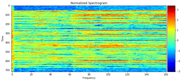
In case of our example the (normalized) spectogram looks like this (this is a waterfall plot):

Mel-Frequency Cepstral Coefficients (MFCC)
Using spectograms has the disadvantage that it covers frequencies we humans cannot hear as well. To reduce dimensionality, we could reduce the spectogram to what we can hear.
This does not only include minimum and maximum frequencies that we can hear but differences between frequencies as well. Btw this concept is used by lossy audio encoders as well.
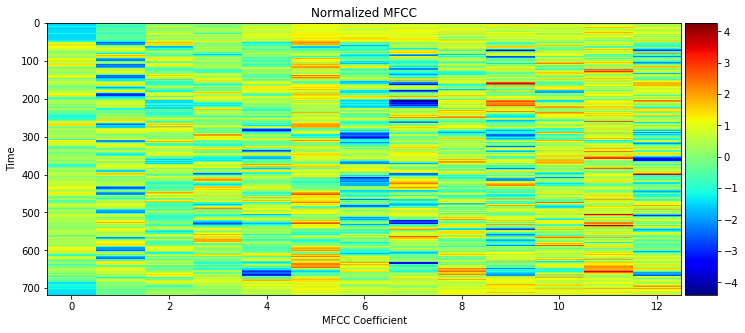
One way to do this is to use the Mel-Frequency Cepstral Coefficients (MFCC). Without going into the details, here is what we get:

RNNs
Audio signals as well as images have a certain structure that should be preserved to make sense of the signal.
Unlike feedforward neural networks, recurrent neural networks (RNNs) preserve the input structure (sequence).
Additionally, speech has not only inherent sequential structure but contextual links as well. But we are not coverying that here in this blog post.
RNNs lead to good performance for such sequential data. Andrej Karpathy wrote a highly recommended blog post on the effectiveness of RNNs.
If we want to use to RNNs, then we have to make a choice between two fundamental units:
- LSTM (Long Short Term Memory)
- GRU (Grated Recurrent Unit)
LSTM (Long Short Term Memory) units
LSTMs are recurrent units that have 3 gates:
- input gate
- output gate
- forget gate.
These gates reguate which information is passed, stored or deleted. We can find a very detailed and excellent but simple explanation of LSTM Networks on colah’s blog.
GRU (Gated Recurrent Unit) units
Gate Recurrent Units are similar to LSTMs but do not have an output gate. This reduces the number of trainable units and therefore perform better on smaller datasets [8].
Model Architectures
We will have a look at a few different model architectures.
Model 1: Single layer RNNs
Model 1 consists of one recurrent layer:
LSTM on spectogram data:
Layer (type)                 Output Shape              Param #
=================================================================
the_input (InputLayer)       (None, None, 161)         0
_________________________________________________________________
rnn (LSTM)                   (None, None, 200)         289600
_________________________________________________________________
bn_simp_rnn (BatchNormalizat (None, None, 200)         800
_________________________________________________________________
time_distributed_1 (TimeDist (None, None, 29)          5829
_________________________________________________________________
softmax (Activation)         (None, None, 29)          0
=================================================================
Total params: 296,229
Trainable params: 295,829
Non-trainable params: 400
_________________________________________________________________
None
Even with a single layer, we experience big differences in the number of trainable parameters:
| Feature | LSTM | GRU |
|---|---|---|
| Spectogram | 295,829 | 223,429 |
| MFCC | 177,429 | 134,629 |
Model 2: 1 Layer CNN and 1 layer RNNs
Model 2 is similar to model 1 but has a 1D convolutional layer with batch normalization before the RNN layer.
We can see that more parameters must be trained:
| Feature | LSTM | GRU |
|---|---|---|
| Spectogram | 681,829 | 601,629 |
| MFCC | 356,229 | 276,029 |
Model 3: Deep RNNs
The deeper RNNs consists of various layers with different units of recurrent units followed by batch normalization.
An example looks like this:
Layer (type)                 Output Shape              Param #
=================================================================
the_input (InputLayer)       (None, None, 161)         0
_________________________________________________________________
lstm_1 (LSTM)                (None, None, 200)         289600
_________________________________________________________________
batch_normalization_1 (Batch (None, None, 200)         800
_________________________________________________________________
lstm_2 (LSTM)                (None, None, 200)         320800
_________________________________________________________________
batch_normalization_2 (Batch (None, None, 200)         800
_________________________________________________________________
time_distributed_1 (TimeDist (None, None, 29)          5829
_________________________________________________________________
softmax (Activation)         (None, None, 29)          0
=================================================================
Total params: 617,829
Trainable params: 617,029
Non-trainable params: 800
_________________________________________________________________
None
Model 4: 1 Layer Bidirectional RNNs
Model 4 consists of one bidirectional RNN unit:
Layer (type)                 Output Shape              Param #
=================================================================
the_input (InputLayer)       (None, None, 161)         0
_________________________________________________________________
bidirectional_1 (Bidirection (None, None, 400)         579200
_________________________________________________________________
bn_rnn_layer_1 (BatchNormali (None, None, 400)         1600
_________________________________________________________________
time_distributed_6 (TimeDist (None, None, 29)          11629
_________________________________________________________________
softmax (Activation)         (None, None, 29)          0
=================================================================
Total params: 592,429
Trainable params: 591,629
Non-trainable params: 800
_________________________________________________________________
None
Model 5: 4 Layer Bidirectional GRUs
Model 4 consists of 4 layers of bidirectional GRUs with 200 units. Unlike previous models it uses dropout as well:
_________________________________________________________________
Layer (type)                 Output Shape              Param #
=================================================================
the_input (InputLayer)       (None, None, 13)          0
_________________________________________________________________
bidirectional_9 (Bidirection (None, None, 400)         256800
_________________________________________________________________
bn_rnn_layer_1 (BatchNormali (None, None, 400)         1600
_________________________________________________________________
bidirectional_10 (Bidirectio (None, None, 400)         721200
_________________________________________________________________
bn_rnn_layer_2 (BatchNormali (None, None, 400)         1600
_________________________________________________________________
bidirectional_11 (Bidirectio (None, None, 400)         721200
_________________________________________________________________
bn_rnn_layer_3 (BatchNormali (None, None, 400)         1600
_________________________________________________________________
bidirectional_12 (Bidirectio (None, None, 400)         721200
_________________________________________________________________
bn_rnn_layer_4 (BatchNormali (None, None, 400)         1600
_________________________________________________________________
time_distributed_3 (TimeDist (None, None, 29)          11629
_________________________________________________________________
softmax (Activation)         (None, None, 29)          0
=================================================================
Total params: 2,438,429
Trainable params: 2,435,229
Non-trainable params: 3,200
_________________________________________________________________
None
Results
Well, lets have a look at the results:
The first thing that we can notice is that using MFCC features and GRUs as recurrent units lead to a lower validation loss with the same amount of epochs as would a model using LSTMs and spectograms.
As far as we can tell from the validation loss graphs we sometimes hit the point where it began to overfit and we would need a different model architecture or much more data.
Using a CNN layer leads to faster convergence to a minimum validation loss with the tendency to overfitting after 10 epochs. There are reports [9] that the performance varies highly with batch sizes. This might be the reason for it. Perhaps the CNN layer oversimplyfies the input for GRU/LSTM too much.
With increasing RNN layers while maintaining the same number of units per layer the differences between using RAW input and MFCC are becoming smaller. This could be caused by the increased amount of trainable parameters. Differences should be minimized over many layers
If we simply increase the number of units but leave the number of layers untouched, then it looks like there is a sweet spot around 200 - 300 units per layer. Less as well as more units will lead to less performance on the same number of epochs. Less units might be not enough to fit the data and more units maight cause overfitting to the training data. Perhaps the dataset is too small for this kind of experimentations. As far as we can tell are MFCC features is less sensitive to the number of units.
Using bidirectional layers lead to better performance but also much longer training times.
So far the model with the 4 bidirectional GRU layer on MFCC features performs best.
Final sanity check
Comparing (ridiculous high) losses with each other is one thing, but let us have a look at sample output of the model:
--------------------------------------------------
True transcription:

the bogus legislature numbered thirty six members
--------------------------------------------------
Here is what we get with model 5:
--------------------------------------------------
Predicted transcription:

the be his legis slater neberd pertysecmevbers
--------------------------------------------------
Back to the drawing board…
If I have time and some free computation time, then I will expand this testing on RNNs quite extensively. I am planning to increase minibatch sizes as well as the numbers of epochs and play around with more model architectures. Further, I am thinking about exploring TCNs (Temporal Convolutional Networks) as well “normal” cov nets.
References
[1] Amodei et al. (2015): Deep Speech 2: End-to-End Speech Recognition in English and Mandarin. online available at: https://arxiv.org/abs/1512.02595.
[2] Panayotov, V.; Chen, G.; Povey, D.; Khudanpur, S. (2015): LibriSpeech: an ASR corpus based on public domain audio books. ICASSP 2015. Preprint available at: http://www.danielpovey.com/files/2015_icassp_librispeech.pdf.
[3] Engel et al. (2017): Neural Audio Synthesis of Musical Notes with WaveNet Autoencoders. Preprint available at: https://arxiv.org/abs/1704.01279v1.
[4] Sainath, T. N. et al. (2015): Learning the speech front-end with raw waveform CLDNNs. Online available at: https://www.semanticscholar.org/paper/Learning-the-speech-front-end-with-raw-waveform-Sainath-Weiss/a566cd4a8623d661a4931814d9dffc72ecbf63c4.
[5] Sainath, T. N. et al. (2017): Multichannel Signal Processing With Deep Neural Networks for Automatic Speech Recognition. doi: 10.1109/TASLP.2017.2672401.
[6] van den Oord et al. (2016): WaveNet: A Generative Model for Raw Audio. Preprint available at: https://arxiv.org/abs/1609.03499v2.
[7] van den Oord et al. (2017): Parallel WaveNet: Fast High-Fidelity Speech Synthesis. Preprint available at: https://arxiv.org/abs/1711.10433v1.
[8] Chung, J.; Gulcehre, C.; Cho, K.H.; Bengio, Y. (2014): “Empirical Evaluation of Gated Recurrent Neural Networks on Sequence Modeling”. Preprint available at: https://arxiv.org/abs/1412.3555.
[9] Yin et al. 2017: Comparative Study of CNN and RNN for Natural Language Processing. Preprint available at: https://arxiv.org/abs/1702.01923.