Contents
Introduction to the Kuzushiji dataset
Kuzushiji is a MNIST-like datasets released in 2018. Unlike most dataset walk-throughs this one is done in Julia. If you like MNIST-like datasets, then have a look at CMNIST as well.
The Kuzushiji dataset [1] is a MNIST-like dataset that contains 10 (Kuzushiji-MNIST) and 49 (Kuzushiji-49) phonetic letters of hiragana. This is a compnent of the Japanese writing system. The intention of the Kuzushiji dataset is link hiragana from classical literature to modern counterparts (UTF-8 encoded). Further, there exists Kuzushiji-Kanji which is a set samples of Kanji which are adopted Chinese characters. All three datasets are based on the Kuzushiji dataset by the National Institute of Japanese Literature. The dataset is licensed under CC BY-SA 4.0.
Since I don’t understand the example images on Hiragana and Kanji, here are my own dataset visualizations. Further, I think that even a classifier with 5 % accuracy outsmarts me and many other people that never had any contact with classical japanese literature. Therefore, it is difficult to look at the data to see if X_train and X_test are labeled correctly.
Since I’m not satisfied with existing packages for data exploration with Julia, we’ll have to write some basic helper functions first:
import CSV
import NPZ
import PyPlot
import Gadfly
import Images
function getCategoricalCount(InputArray)
    Count = Dict{Any,Int64}()
    for (Index, Category) in enumerate(InputArray)
        if haskey(Count, Category)
            Count[Category] +=1
        else
            Count[Category] = 1
        end
    end
    return sort(Count)
end
function getCategoricalIndices(InputArray)
    CategoricalIndices = Dict{Any,Array{Int64,1}}()
    for (Index, Category) in enumerate(InputArray)
        if haskey(CategoricalIndices, Category)
            push!(CategoricalIndices[Category], Index)
        else
            CategoricalIndices[Category] = [Index]
        end
    end
    return CategoricalIndices
end
function CollectAllImagesPerCategory(InputArray,CategoricalIndices,NumberOfExamples)
    if NumberOfExamples > size(CategoricalIndices)[1]
        NumberOfExamples = size(CategoricalIndices)[1]
    end
    ItemsXY = convert(Int64,ceil(sqrt(NumberOfExamples)))
    ImageSizeY = size(InputArray)[2]
    ImageSizeX = size(InputArray)[3]
    i = 1
    FirstRow = true
    FirstItemInRow = true
    OutputArrayRow = []
    OutputArray = []
    for j in collect(1:ItemsXY)
        for k in collect(1:ItemsXY)
            if (FirstItemInRow == true)
                OutputArrayRow = InputArray[CategoricalIndices[i],:,:]
                OutputArrayRow = hcat(OutputArrayRow, zeros(ImageSizeY,ImageSizeX))
                FirstItemInRow = false
                i+=1
            elseif (i <= NumberOfExamples)
                OutputArrayRow = hcat(OutputArrayRow,InputArray[CategoricalIndices[i],:,:])
                OutputArrayRow = hcat(OutputArrayRow, zeros(ImageSizeY,ImageSizeX))
                i+=1
            else
                OutputArrayRow = hcat(OutputArrayRow, zeros(ImageSizeY,ImageSizeX * 2))
                i+=1
            end
        end
        FirstItemInRow = true
        if FirstRow == false
            OutputArray = vcat(OutputArray, OutputArrayRow)
            OutputArray = vcat(OutputArray, zeros(ImageSizeY,ImageSizeX*2*ItemsXY))
        else
            OutputArray = zeros(ImageSizeY,ImageSizeX*2*ItemsXY)
            OutputArray = vcat(OutputArray,OutputArrayRow)
            OutputArray = vcat(OutputArray, zeros(ImageSizeY,ImageSizeX*2*ItemsXY))
            FirstRow = false
        end
    end
    return hcat(zeros(size(OutputArray)[1],ImageSizeX),OutputArray)
end
function PlotExampleImagesPerCategory(InputArray, CategoricalIndices, NumberOfExamples,DatasetName)
    for i in collect(keys(CategoricalIndices))
        Examples = CollectAllImagesPerCategory(InputArray,CategoricalIndices[i],NumberOfExamples)
        PyPlot.figure(figsize=(12,12))
        PyPlot.imshow(Examples, cmap="gray")
        PyPlot.title("Examples of class "*string(i)*" of "*DatasetName)
        PyPlot.xticks([])
        PyPlot.yticks([])
        PyPlot.tight_layout()
        PyPlot.savefig("./graphics/"*DatasetName*"_examples_class_"*string(i)*".png")
        PyPlot.close()
    end
end
function PlotHistogram(Categories, Title, XLabel="Class", YLabel="Frequency")
    Plot = Gadfly.plot(x=[string(i) for i in collect(keys(Categories))],
        y=collect(values(Categories)),
        Gadfly.Geom.bar,
        color=[string(i) for i in collect(keys(Categories))],
        Gadfly.Guide.xlabel(XLabel),
        Gadfly.Guide.ylabel(YLabel),
        Gadfly.Guide.title(Title * " Histogram"),
        Gadfly.Guide.colorkey(title=XLabel));
    ImageParams = Gadfly.SVG("./graphics/"*Title*"_histogram.svg", 14Gadfly.cm, 10Gadfly.cm);
    Gadfly.draw(ImageParams, Plot);
end
Kuzushiji-MNIST
The Kuzushiji-MNIST or KMNIST dataset contains 10 classes of hiragana characters with a resolution of 28x28 (grayscale) similar to MNIST. In total it contains 70k images, 60k for training and 10k for testing.
Let’s have a look what characters are contained in KMNIST:
ClassLabels_Kuzushiji_MNIST = CSV.File("./Kuzushiji-MNIST/data/kmnist_classmap.csv") |> CSV.DataFrame
nb!: by default Julia uses index 1 and not index 0
| index | target value | codepoint | char |
|---|---|---|---|
| 1 | 0 | U+304A | お |
| 2 | 1 | U+304D | き |
| 3 | 2 | U+3059 | す |
| 4 | 3 | U+3064 | つ |
| 5 | 4 | U+306A | な |
| 6 | 5 | U+306F | は |
| 7 | 6 | U+307E | ま |
| 8 | 7 | U+3084 | や |
| 9 | 8 | U+308C | れ |
| 10 | 9 | U+3092 | を |
Kuzushiji_MNIST_X_train = NPZ.npzread("./Kuzushiji-MNIST/data/kmnist-train-imgs.npz")["arr_0"];
Kuzushiji_MNIST_X_test = NPZ.npzread("./Kuzushiji-MNIST/data/kmnist-test-imgs.npz")["arr_0"];
Kuzushiji_MNIST_y_train = NPZ.npzread("./Kuzushiji-MNIST/data/kmnist-train-labels.npz")["arr_0"];
Kuzushiji_MNIST_y_test = NPZ.npzread("./Kuzushiji-MNIST/data/kmnist-test-labels.npz")["arr_0"];
The first entry in the training set is supposed to be classified as “8” (れ) and looks like this as an array:
28×28 Array{UInt8,2}:
0x00 0x00 0x00 0x00 0x00 0x00 … 0x00 0x00 0x00 0x00 0x00 0x00
0x00 0x00 0x00 0x00 0x00 0x00 0x00 0x00 0x00 0x00 0x00 0x00
0x00 0x00 0x00 0x00 0x00 0x00 0x00 0x00 0x00 0x00 0x00 0x00
0x00 0x00 0x00 0x00 0x00 0x00 0x00 0x00 0x00 0x00 0x00 0x00
0x00 0x00 0x00 0x00 0x00 0x00 0x00 0x00 0x00 0x00 0x00 0x00
0x00 0x00 0x00 0x00 0x00 0x00 … 0x00 0x00 0x00 0x00 0x00 0x00
0x00 0x00 0x00 0x00 0x00 0x00 0x00 0x00 0x00 0x00 0x00 0x00
0x00 0x00 0x00 0x00 0x00 0x00 0x00 0x00 0x00 0x00 0x00 0x00
⋮ ⋮ ⋱ ⋮
0x00 0x00 0x00 0x00 0x00 0x00 0x00 0x00 0x00 0x00 0x00 0x00
0x00 0x00 0x00 0x00 0x00 0x00 0x00 0x00 0x00 0x00 0x00 0x00
0x00 0x00 0x00 0x00 0x00 0x00 0x00 0x00 0x00 0x00 0x00 0x00
0x00 0x00 0x00 0x00 0x00 0x00 0x00 0x00 0x00 0x00 0x00 0x00
0x00 0x00 0x00 0x00 0x00 0x00 … 0x00 0x00 0x00 0x00 0x00 0x00
0x00 0x00 0x00 0x00 0x00 0x00 0x00 0x00 0x00 0x00 0x00 0x00
0x00 0x00 0x00 0x00 0x00 0x00 0x00 0x00 0x00 0x00 0x00 0x00
0x00 0x00 0x00 0x00 0x00 0x00 0x00 0x00 0x00 0x00 0x00 0x00
0x00 0x00 0x00 0x00 0x00 0x00 0x00 0x00 0x00 0x00 0x00 0x00
0x00 0x00 0x00 0x00 0x00 0x00 … 0x00 0x00 0x00 0x00 0x00 0x00
0x00 0x00 0x00 0x00 0x00 0x00 0x00 0x00 0x00 0x00 0x00 0x00
0x00 0x00 0x00 0x00 0x00 0x00 0x00 0x00 0x00 0x00 0x00 0x00
nb!: Julia stores UInt8 as hexadecimal (base16). If you want to see it (visually) in base10, then you would have to convert it to Int16: convert(Array{Int16,3},NPZ.npzread("./Kuzushiji-MNIST/data/kmnist-train-imgs.npz")["arr_0"]);
We can plot this character using PyPlot:
PyPlot.figure(figsize=(1,1));
PyPlot.imshow(Kuzushiji_MNIST_X_train[1,:,:], cmap="gray");
PyPlot.show();
I have no idea how this can be the same as this modern symbol: れ. But again, this is a modern representation and I don’t know a single thing about Japanese.
Kuzushiji_MNIST_CategoricalCount = getCategoricalCount(Kuzushiji_MNIST_y_train);
Kuzushiji_MNIST_CategoricalIndices = getCategoricalIndices(Kuzushiji_MNIST_y_train);
PlotExampleImagesPerCategory(Kuzushiji_MNIST_X_train, Kuzushiji_MNIST_CategoricalIndices,144, "Kuzushiji-MNIST")
PlotHistogram(Kuzushiji_MNIST_CategoricalCount, "Kuzushiji-MNIST Histogram")
The classes are distributed uniformly. Let’s have a look at a few examples per class:
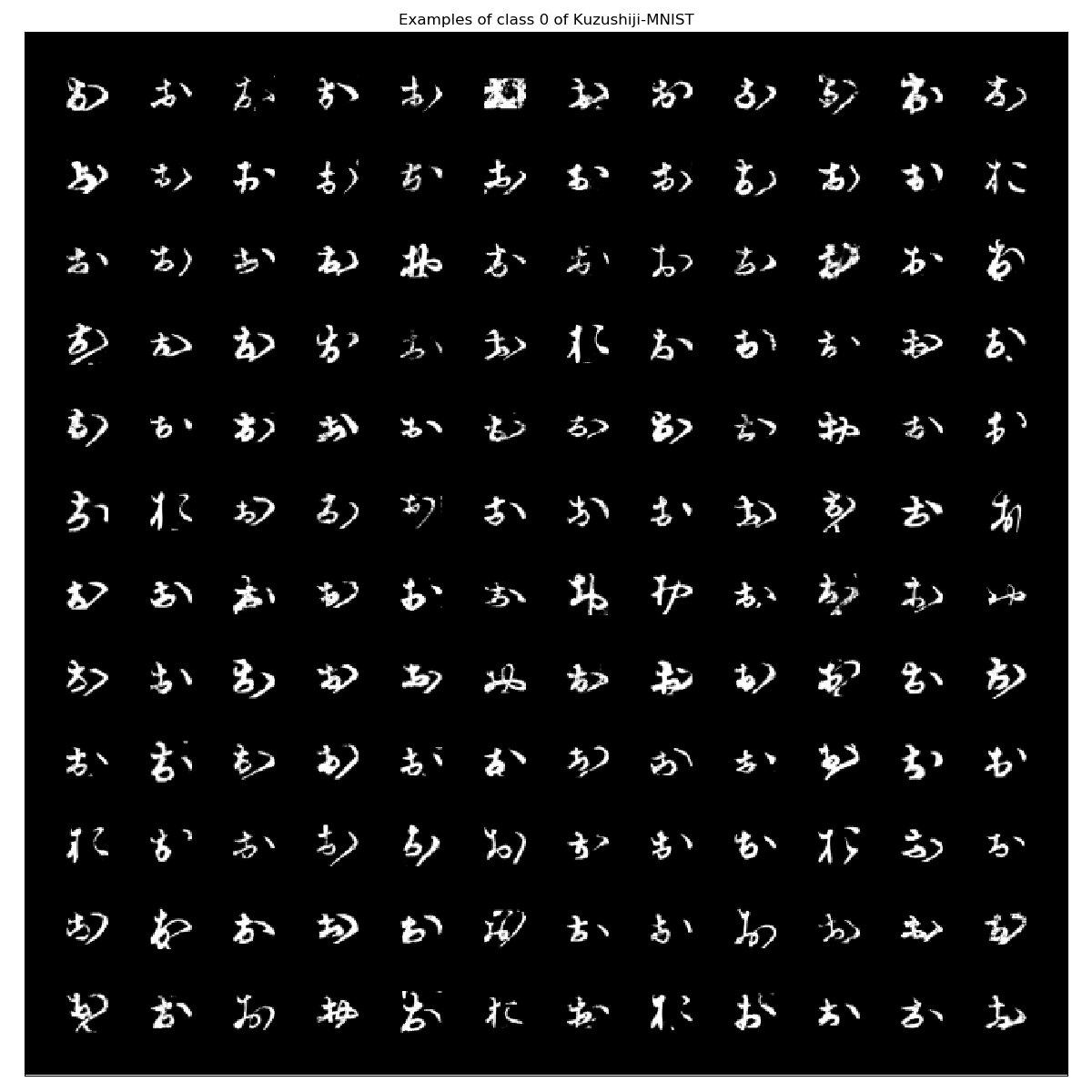

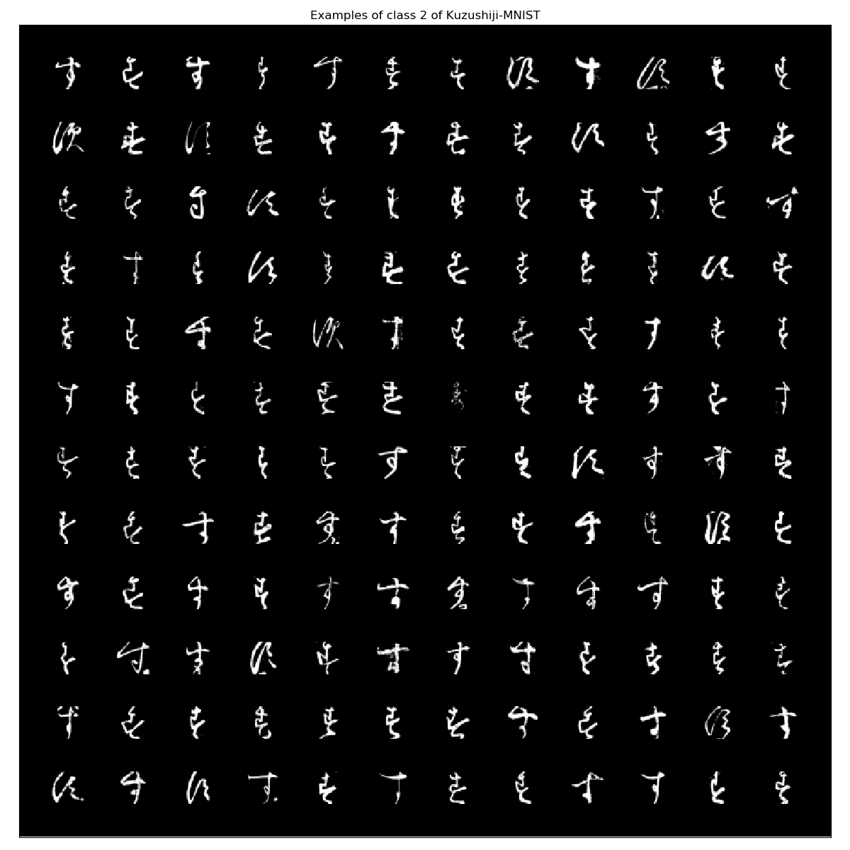
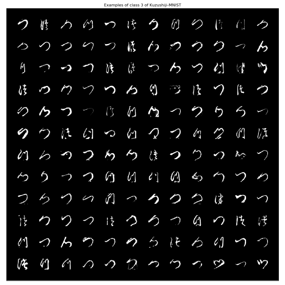
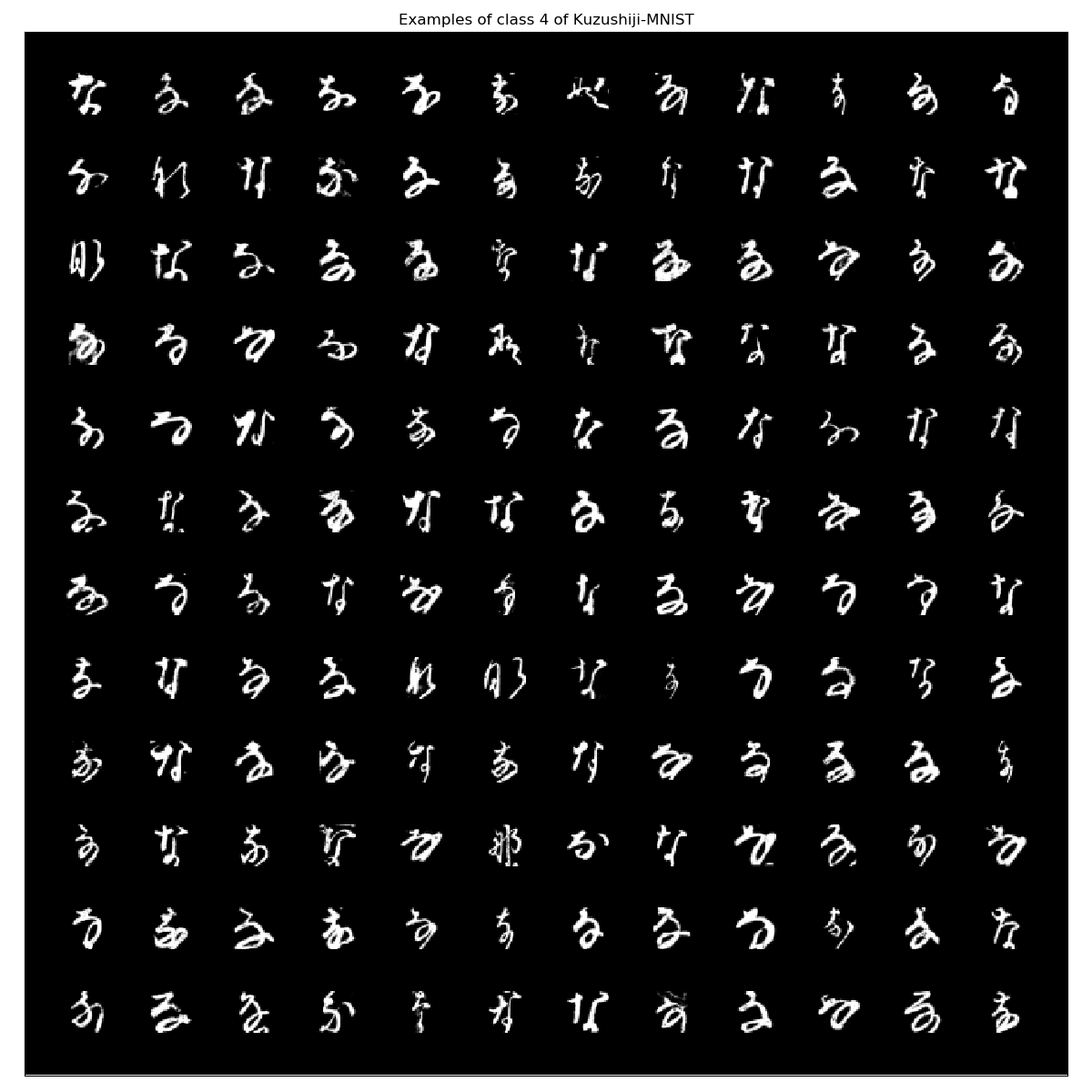
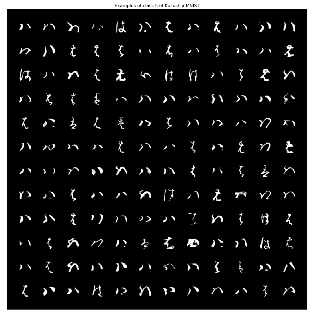
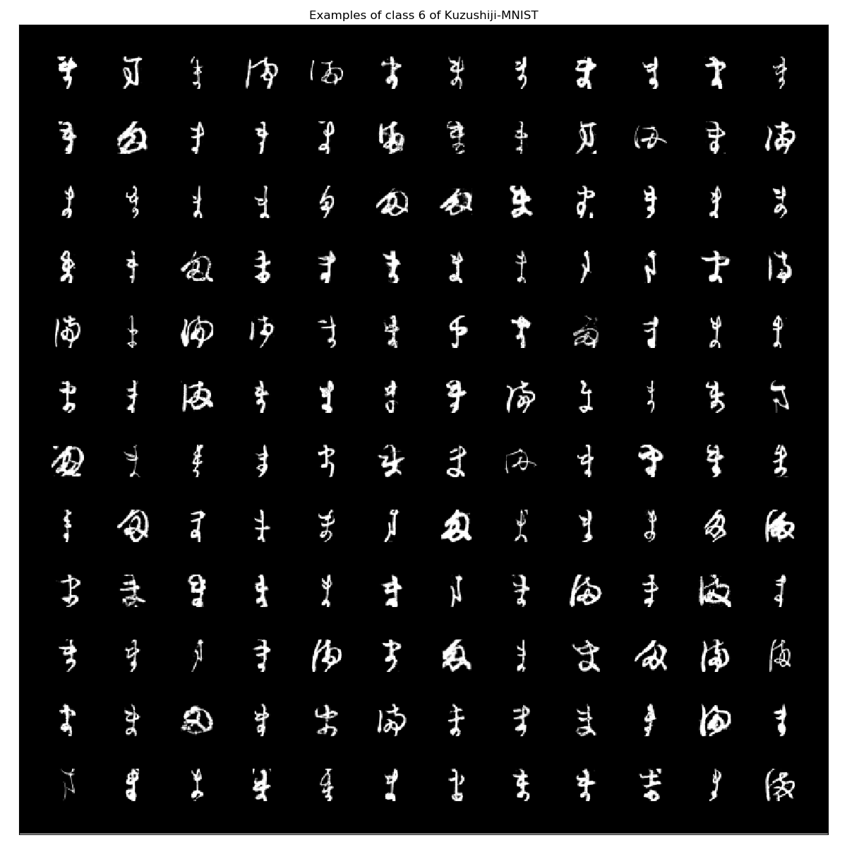
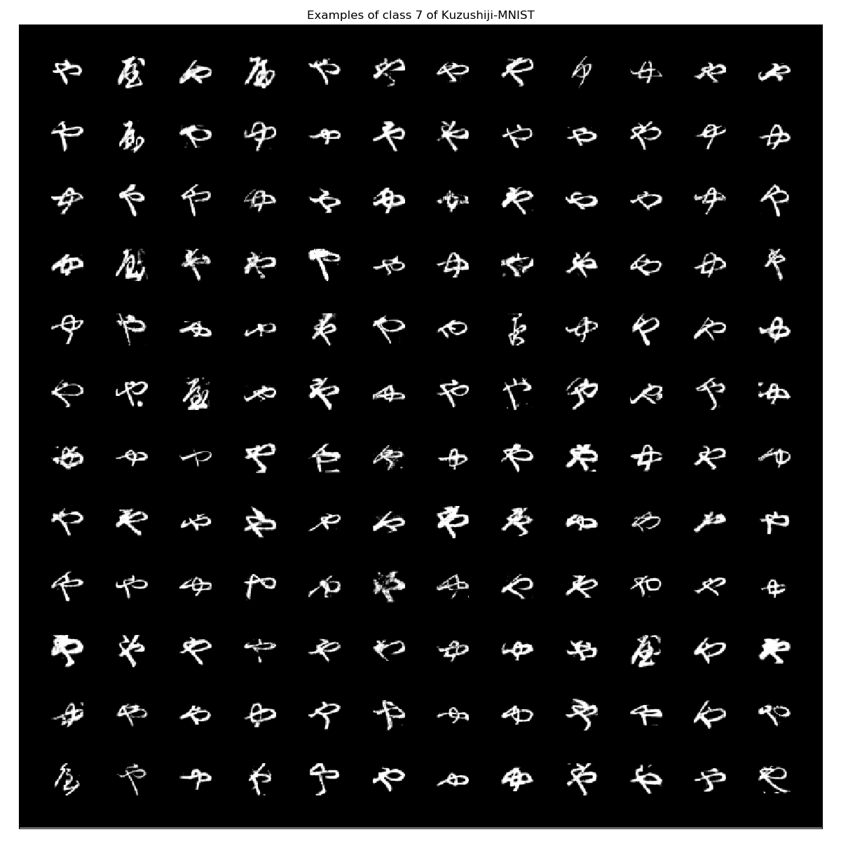
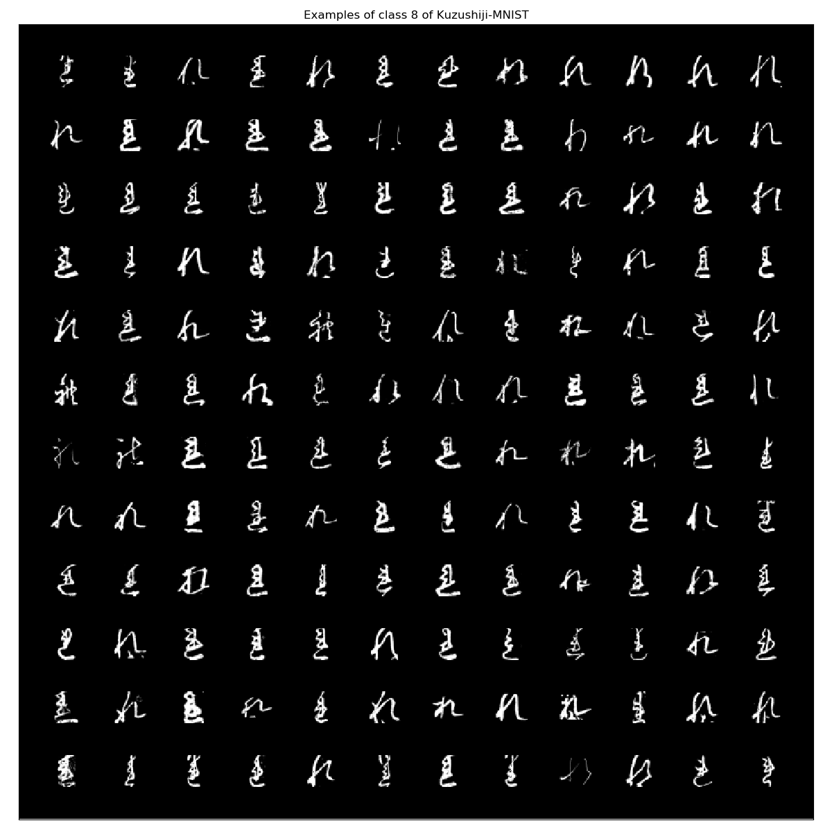
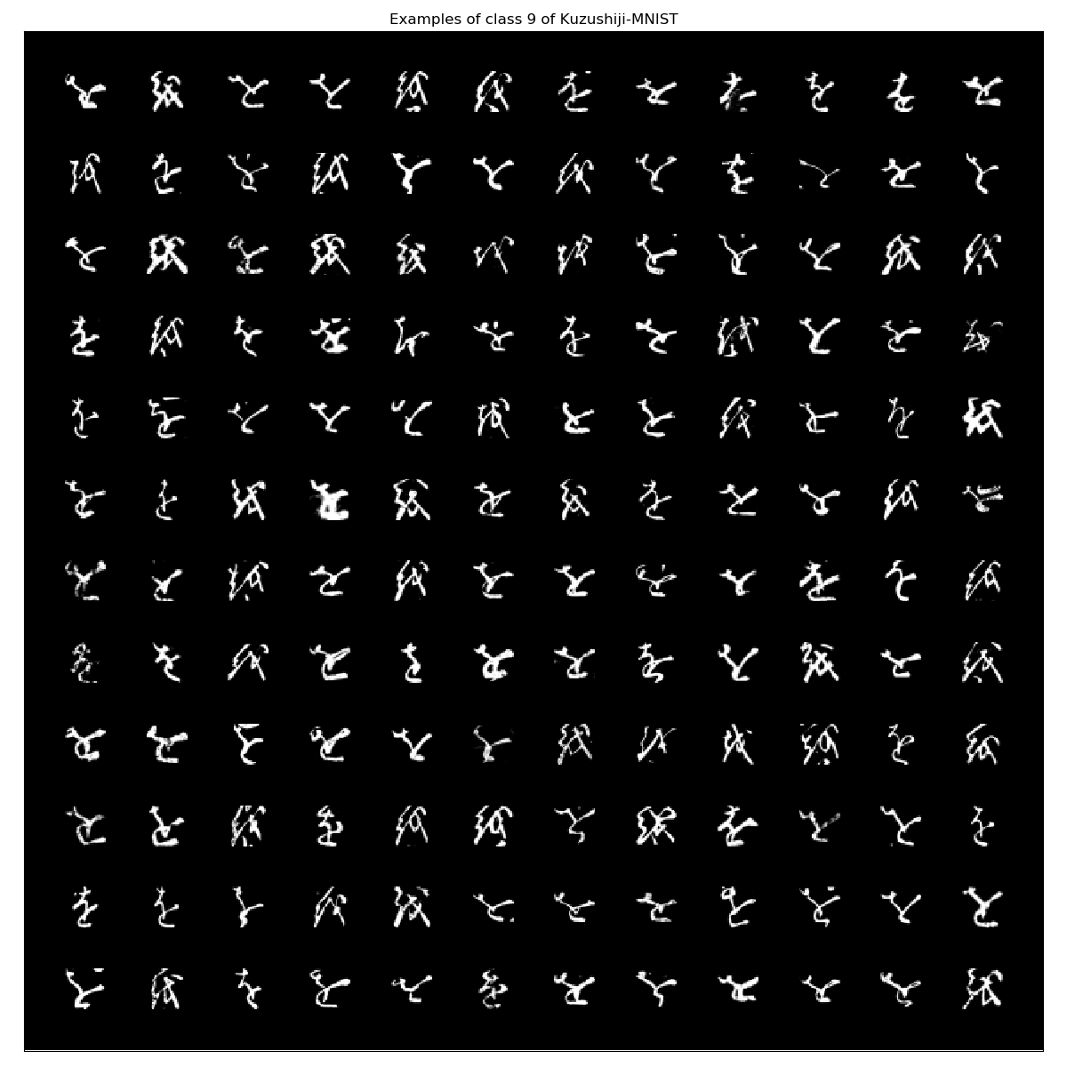
From my point of there are some images that could be misclassified. However, besides detecting basic shapes they all look alike to mee.
Update: the dataset contains some black images: A bug report as been filed already: https://github.com/rois-codh/kmnist/issues/1.
Kuzushiji-49
Kuzushiji-49 is similar to KMNIST. However, it contains 270912 images of 49 classes which are not distributed evenly. It contains images of the following characters:
ClassLabels_Kuzushiji_49 = CSV.File("./Kuzushiji-49/data/k49_classmap.csv") |> CSV.DataFrame
| index | target value | codepoint | char |
|---|---|---|---|
| 1 | 0 | U+3042 | あ |
| 2 | 1 | U+3044 | い |
| 3 | 2 | U+3046 | う |
| 4 | 3 | U+3048 | え |
| 5 | 4 | U+304A | お |
| 6 | 5 | U+304B | か |
| 7 | 6 | U+304D | き |
| 8 | 7 | U+304F | く |
| 9 | 8 | U+3051 | け |
| 10 | 9 | U+3053 | こ |
| 11 | 10 | U+3055 | さ |
| 12 | 11 | U+3057 | し |
| 13 | 12 | U+3059 | す |
| 14 | 13 | U+305B | せ |
| 15 | 14 | U+305D | そ |
| 16 | 15 | U+305F | た |
| 17 | 16 | U+3061 | ち |
| 18 | 17 | U+3064 | つ |
| 19 | 18 | U+3066 | て |
| 20 | 19 | U+3068 | と |
| 21 | 20 | U+306A | な |
| 22 | 21 | U+306B | に |
| 23 | 22 | U+306C | ぬ |
| 24 | 23 | U+306D | ね |
| 25 | 24 | U+306E | の |
| 26 | 25 | U+306F | は |
| 27 | 26 | U+3072 | ひ |
| 28 | 27 | U+3075 | ふ |
| 29 | 28 | U+3078 | へ |
| 30 | 29 | U+307B | ほ |
| 31 | 30 | U+307E | ま |
| 32 | 31 | U+307F | み |
| 33 | 32 | U+3080 | む |
| 34 | 33 | U+3081 | め |
| 35 | 34 | U+3082 | も |
| 36 | 35 | U+3084 | や |
| 37 | 36 | U+3086 | ゆ |
| 38 | 37 | U+3088 | よ |
| 39 | 38 | U+3089 | ら |
| 40 | 39 | U+308A | り |
| 41 | 40 | U+308B | る |
| 42 | 41 | U+308C | れ |
| 43 | 42 | U+308D | ろ |
| 44 | 43 | U+308F | わ |
| 45 | 44 | U+3090 | ゐ |
| 46 | 45 | U+3091 | ゑ |
| 47 | 46 | U+3092 | を |
| 48 | 47 | U+3093 | ん |
| 49 | 48 | U+309D | ゝ |
Kuzushiji_49_X_train = NPZ.npzread("./Kuzushiji-49/data/k49-train-imgs.npz")["arr_0"];
Kuzushiji_49_X_test = NPZ.npzread("./Kuzushiji-49/data/k49-test-imgs.npz")["arr_0"];
Kuzushiji_49_y_train = NPZ.npzread("./Kuzushiji-49/data/k49-train-labels.npz")["arr_0"];
Kuzushiji_49_y_test = NPZ.npzread("./Kuzushiji-49/data/k49-test-labels.npz")["arr_0"];

Kuzushiji_49_CategoricalCount = getCategoricalCount(Kuzushiji_49_y_train);
Kuzushiji_49_CategoricalIndices = getCategoricalIndices(Kuzushiji_49_y_train);
PlotExampleImagesPerCategory(Kuzushiji_49_X_train, Kuzushiji_49_CategoricalIndices,144, "Kuzushiji-49")
PlotHistogram(Kuzushiji_49_CategoricalCount, "Kuzushiji-49 Histogram")
The examples of each class look like this:
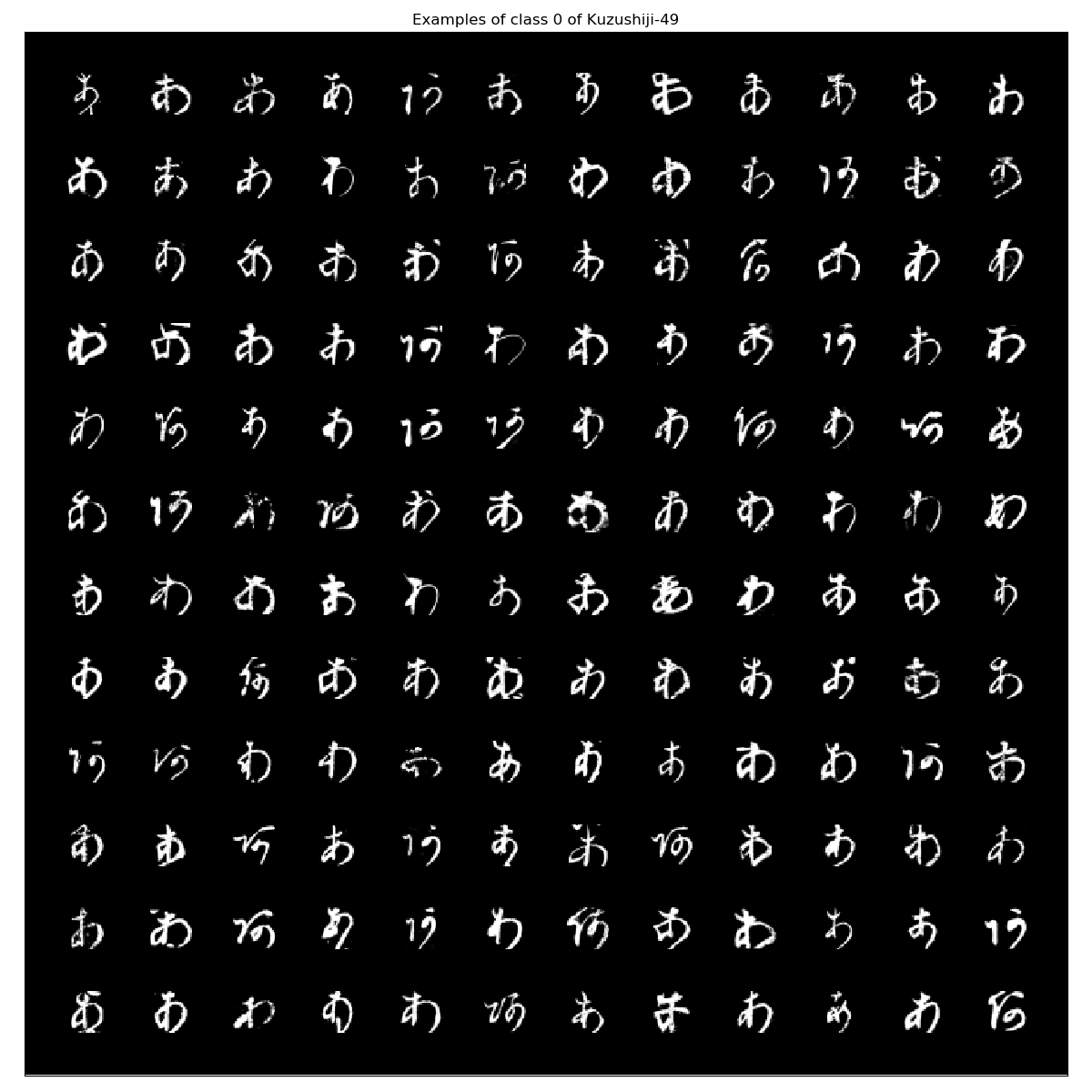
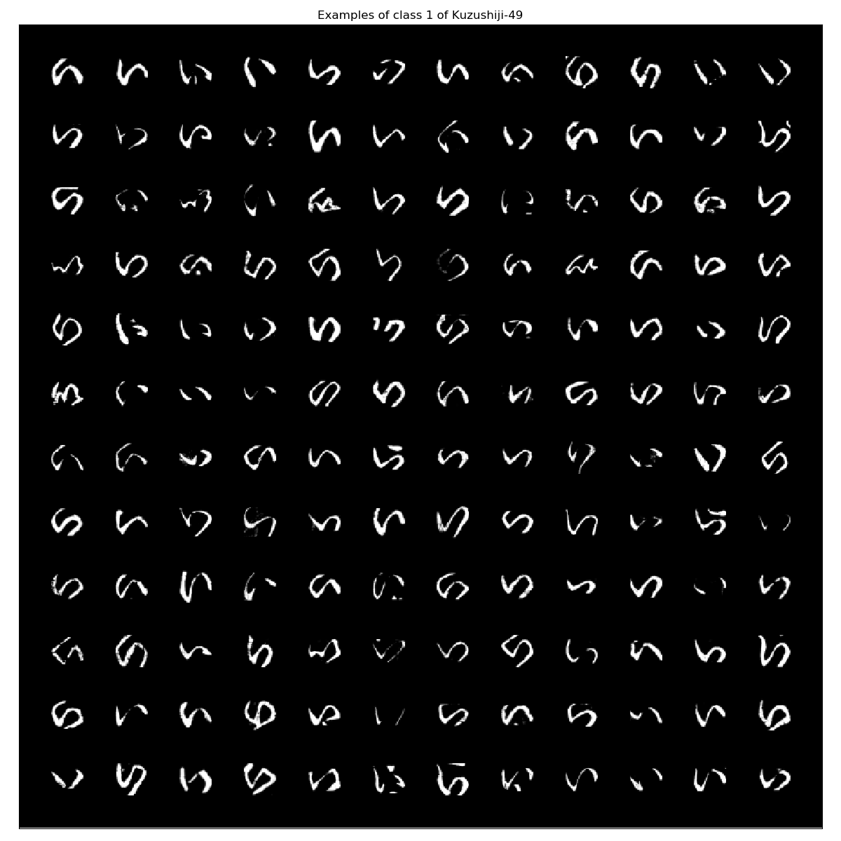
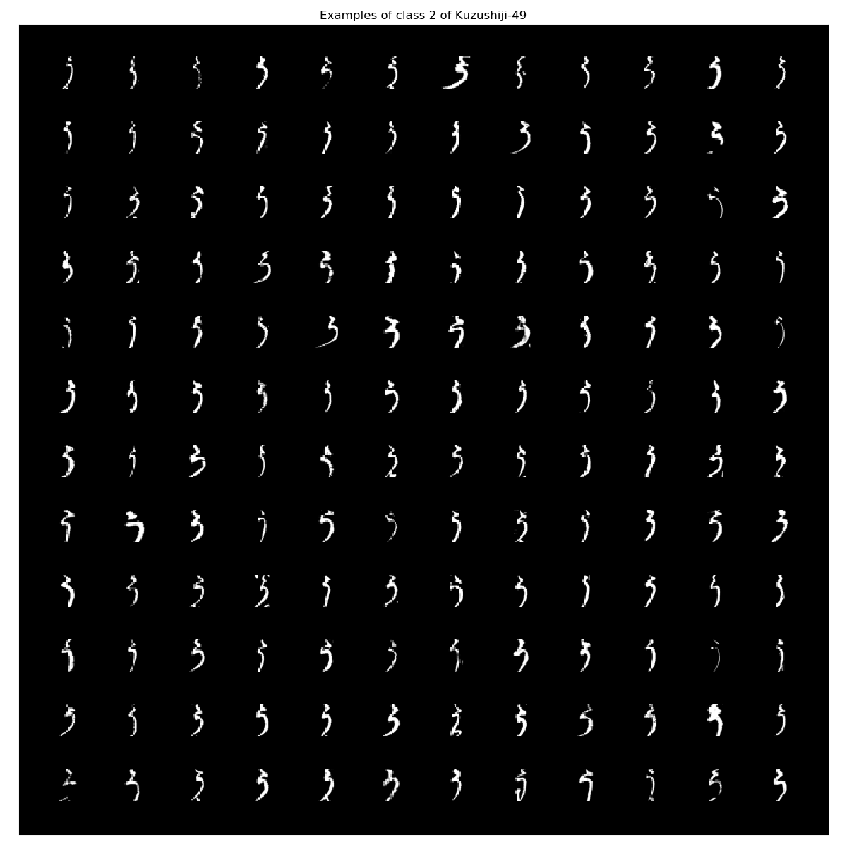
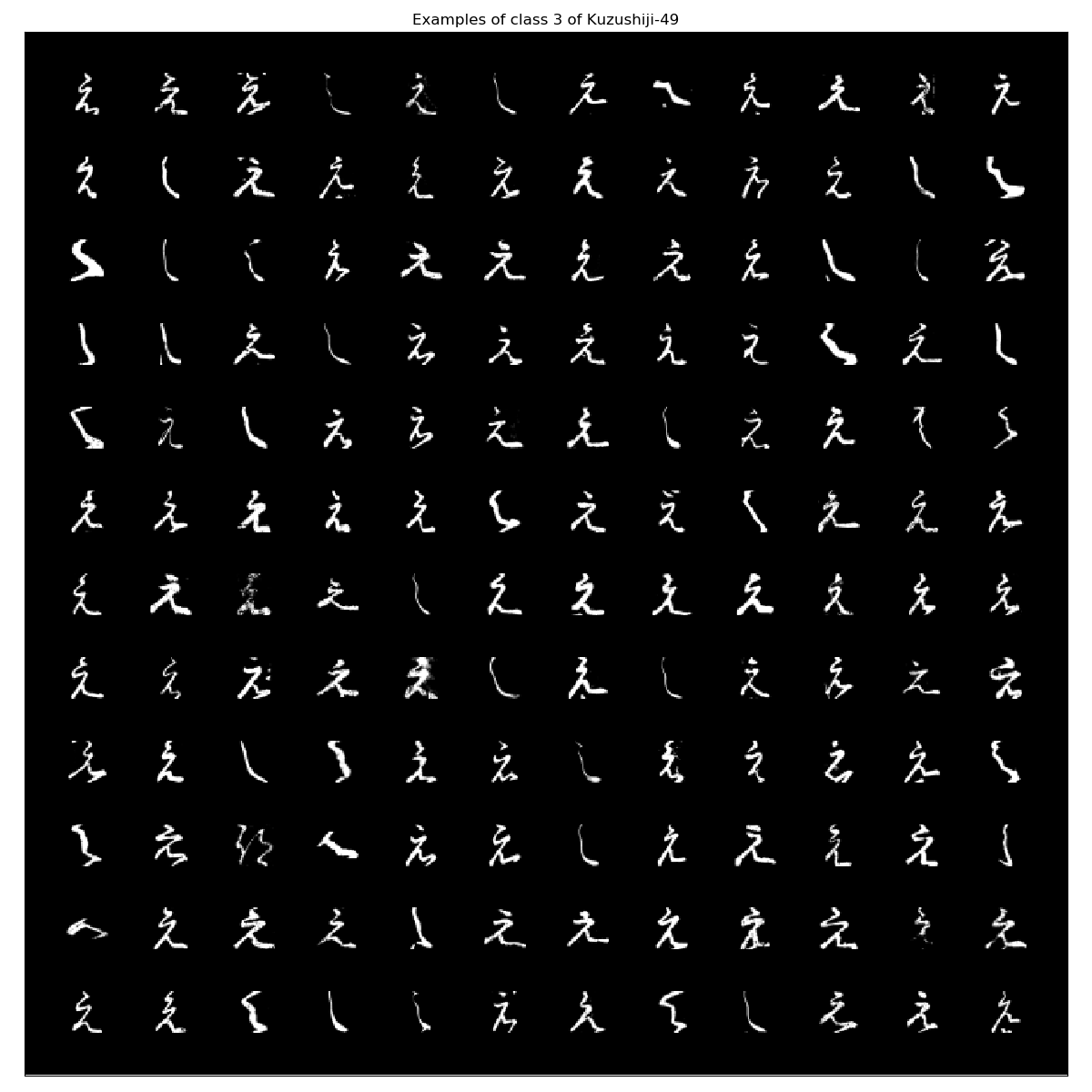
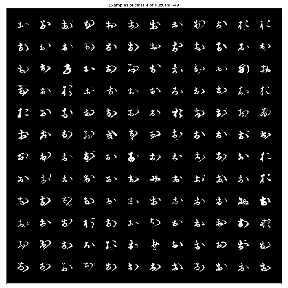
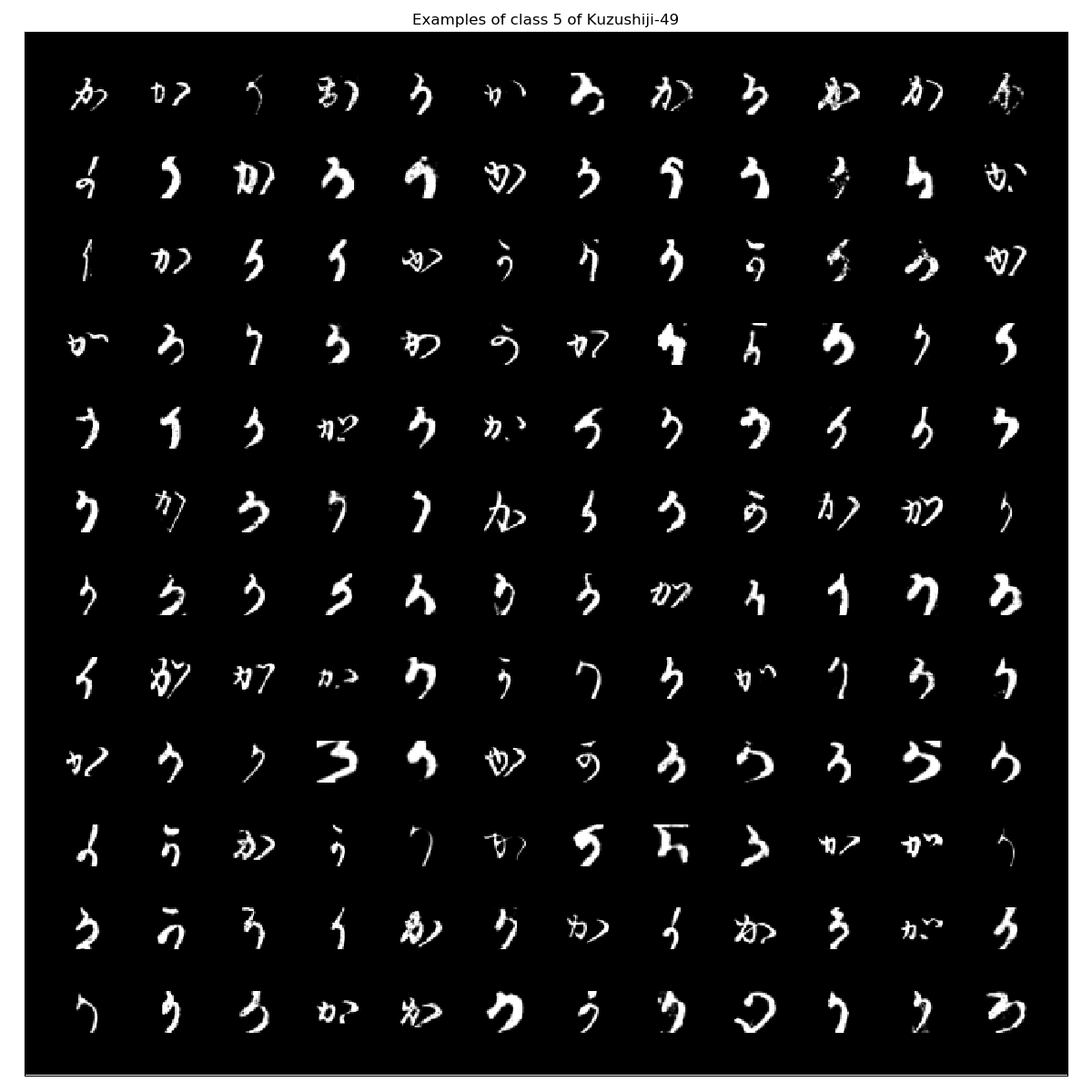
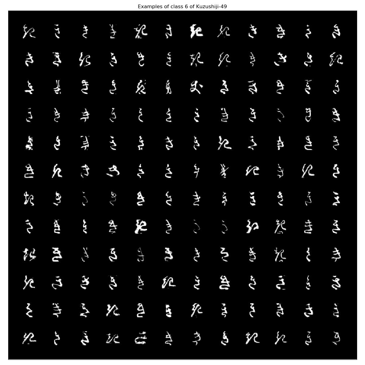
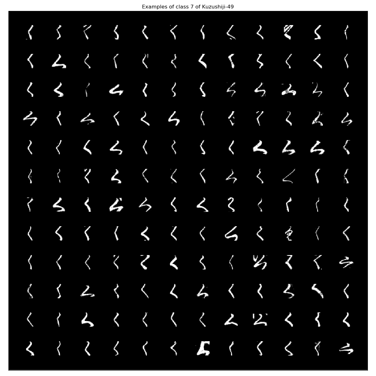
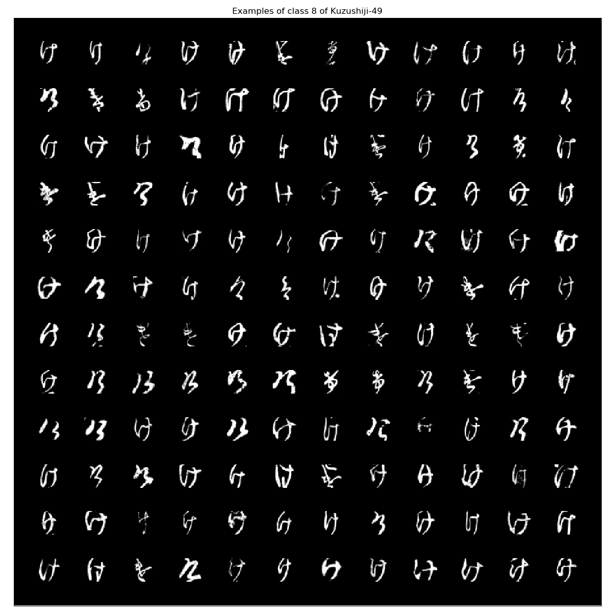
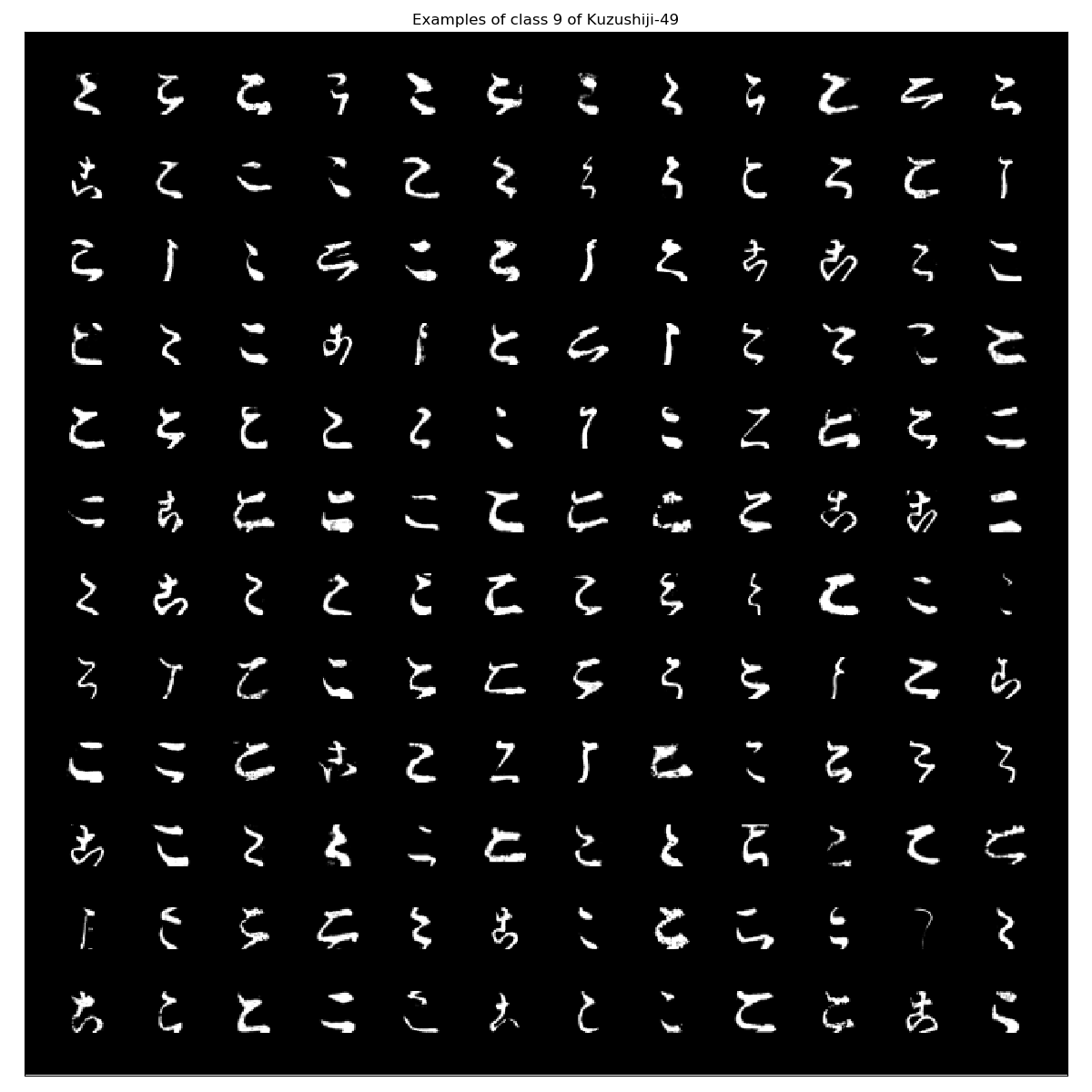
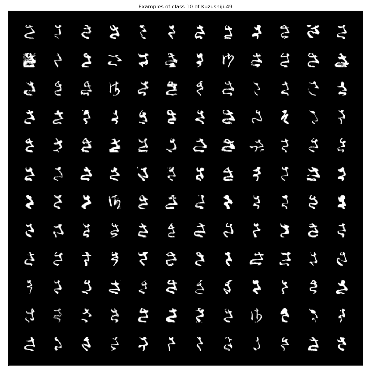
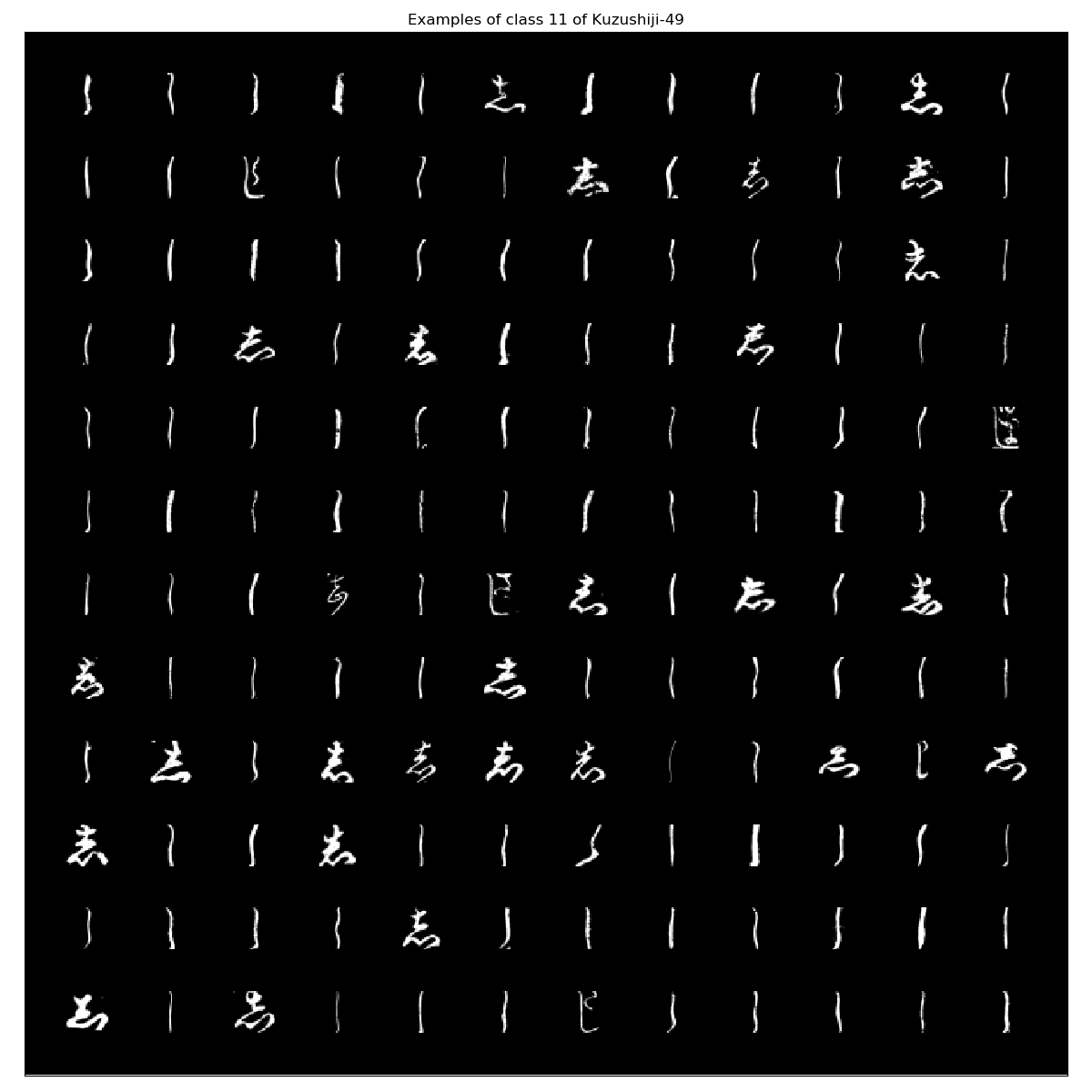
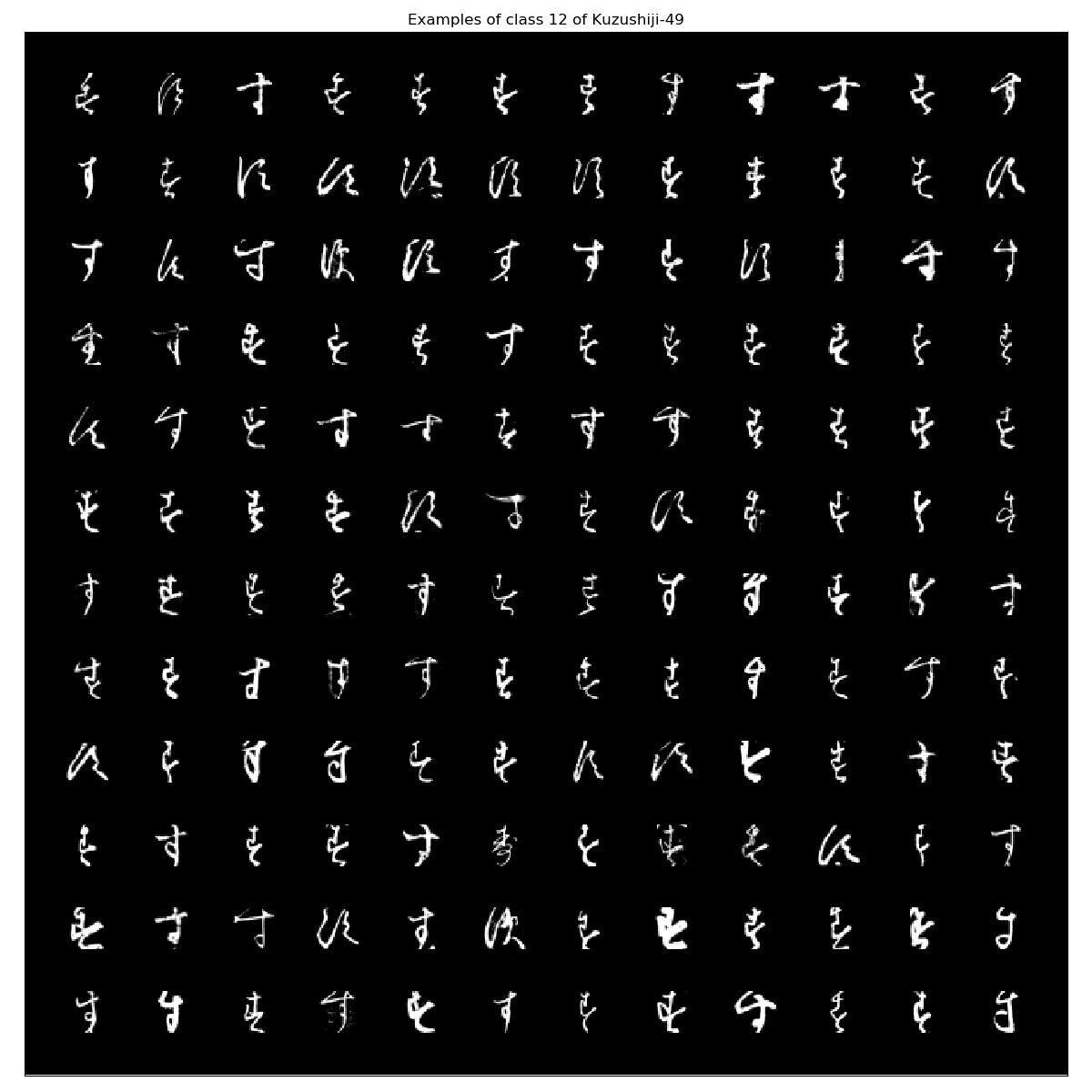
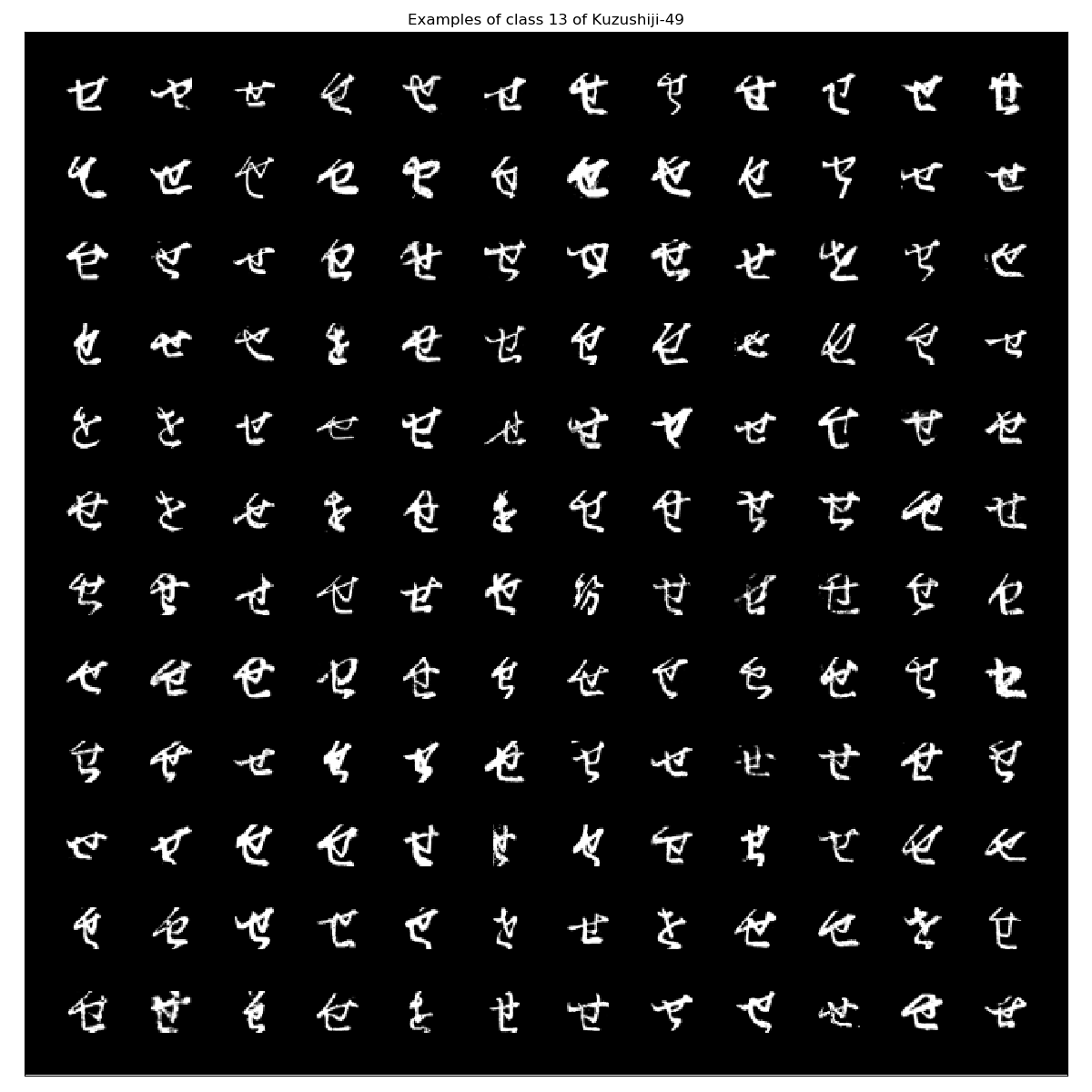
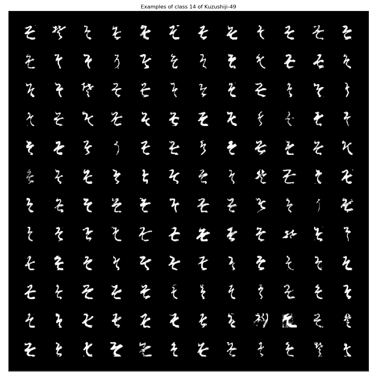
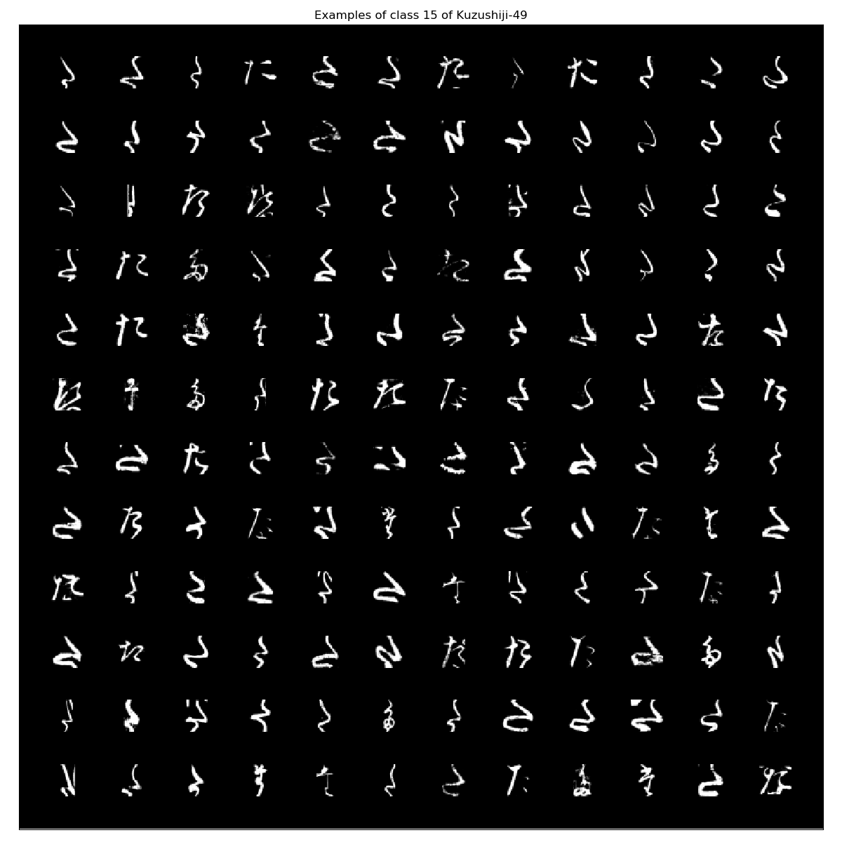
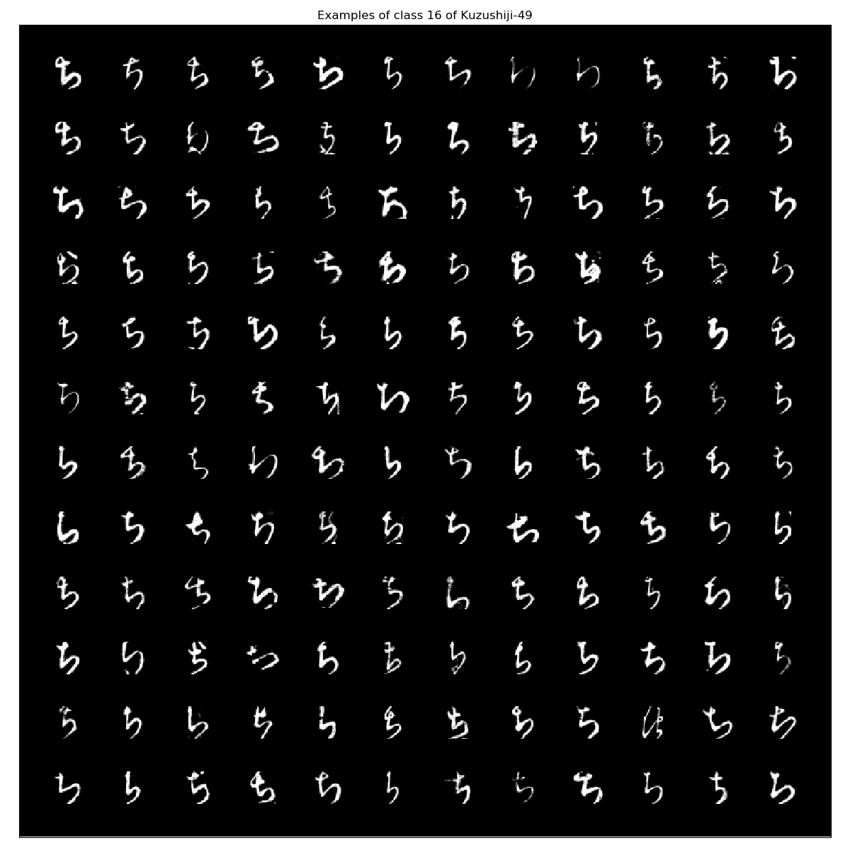
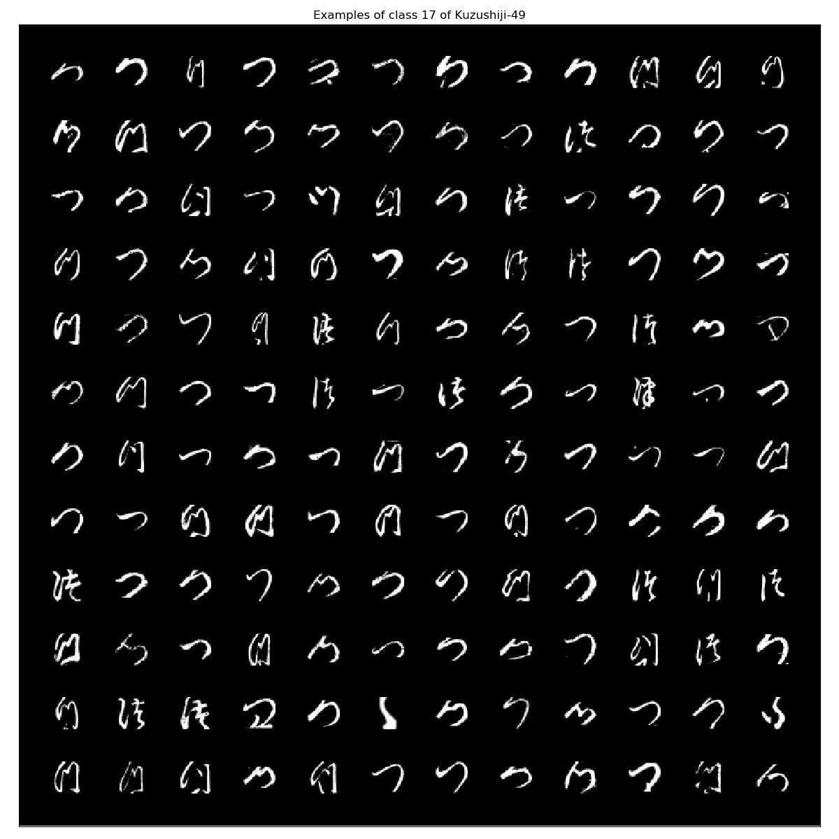
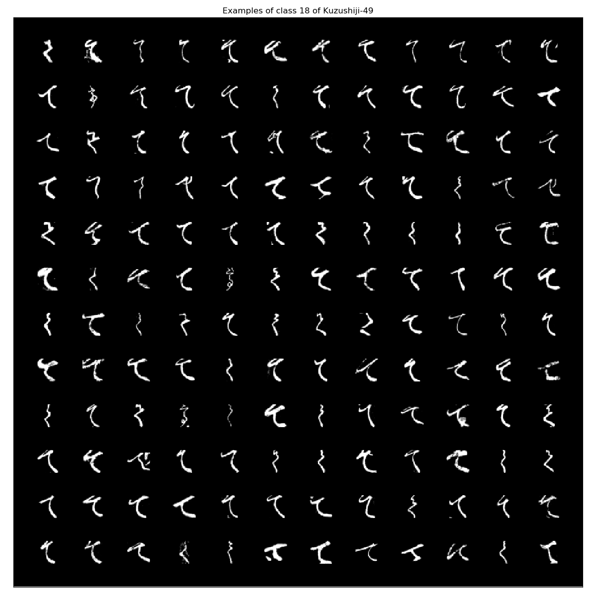
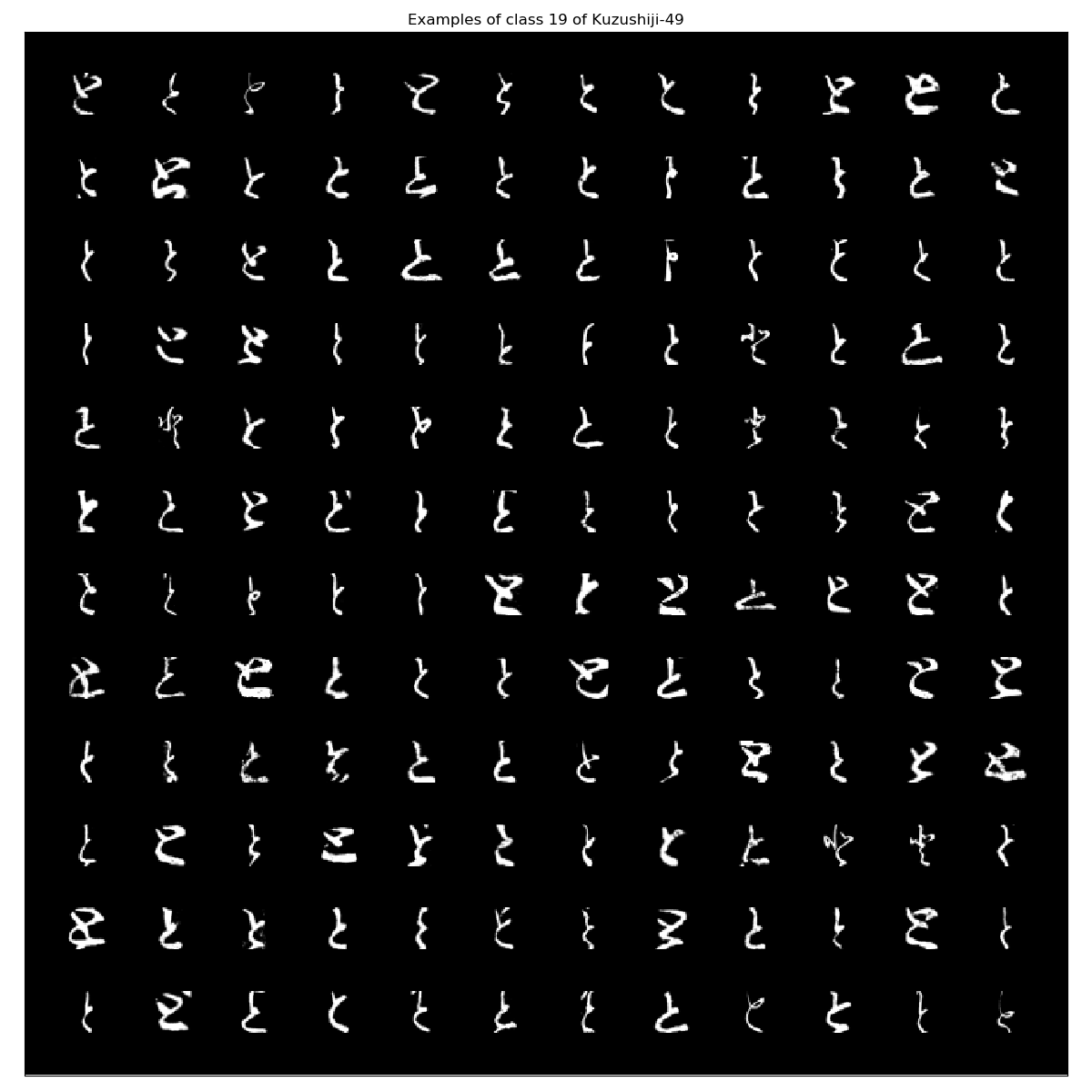
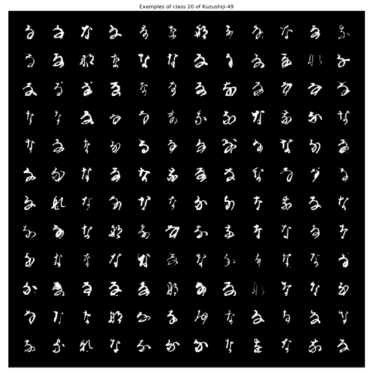
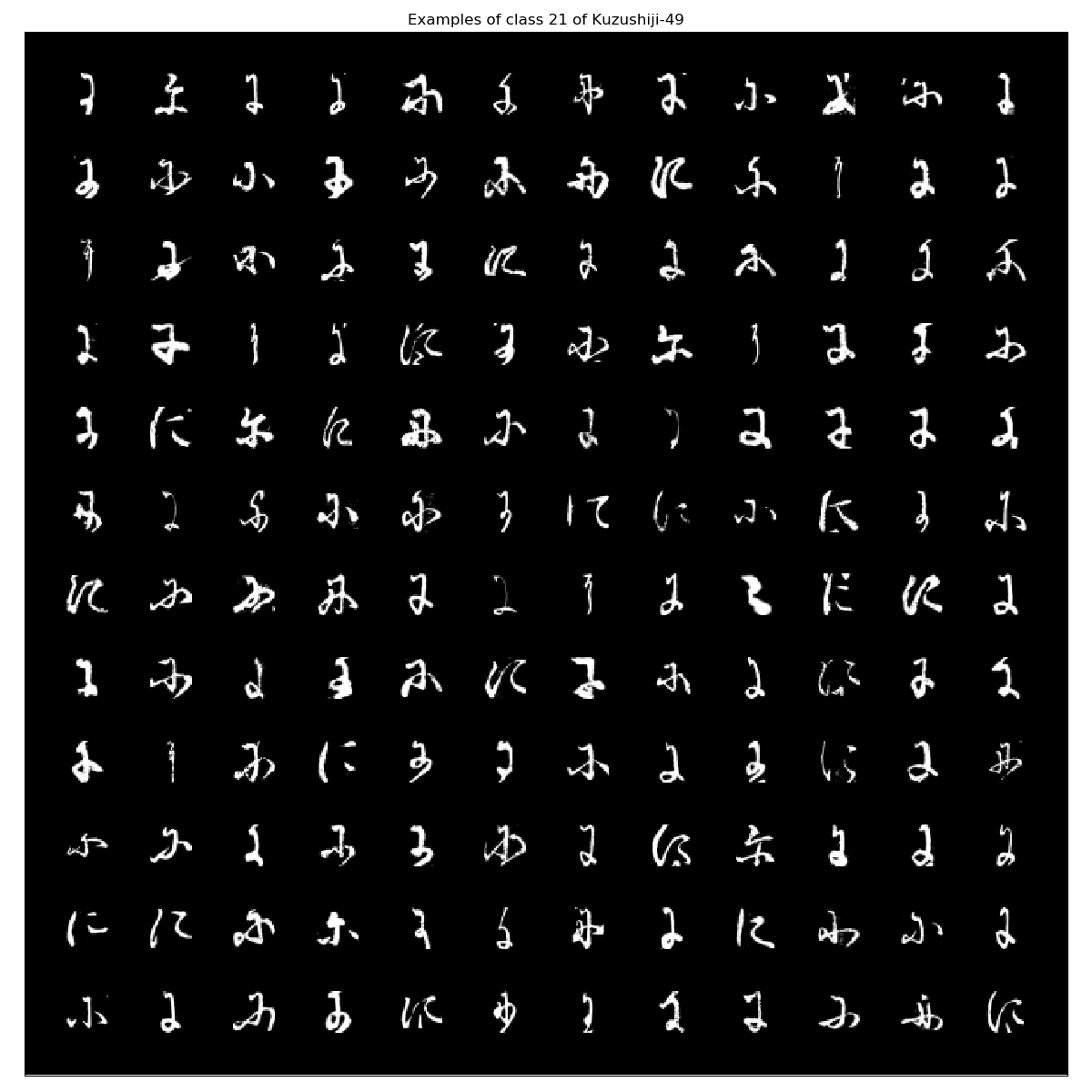
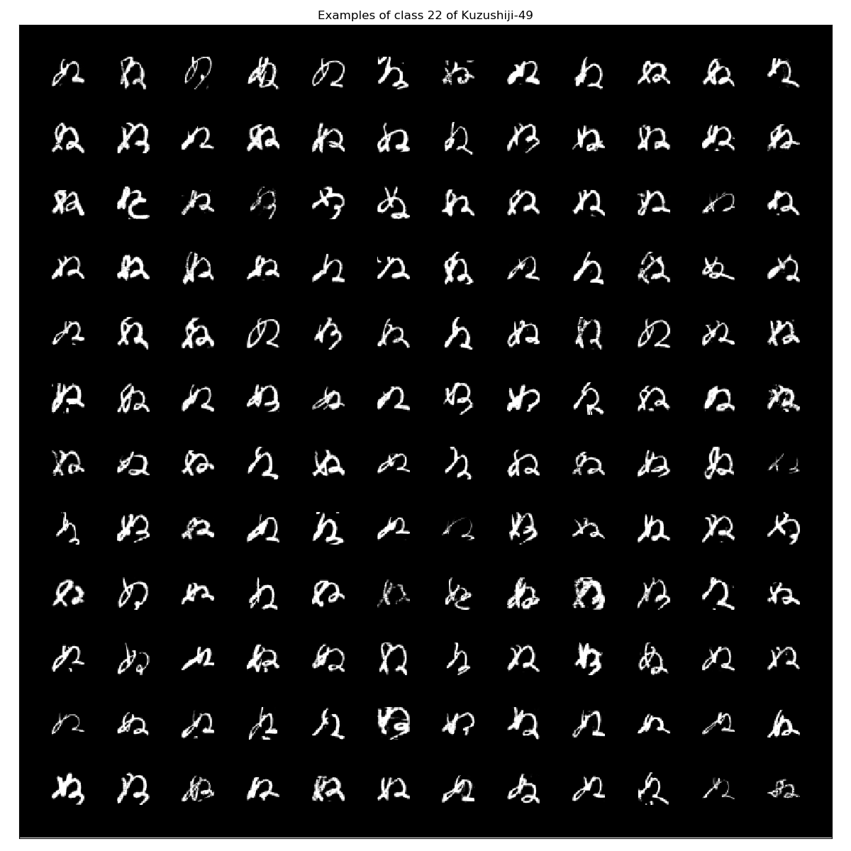
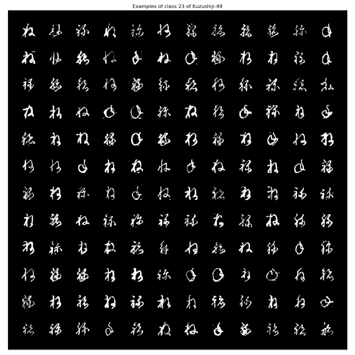
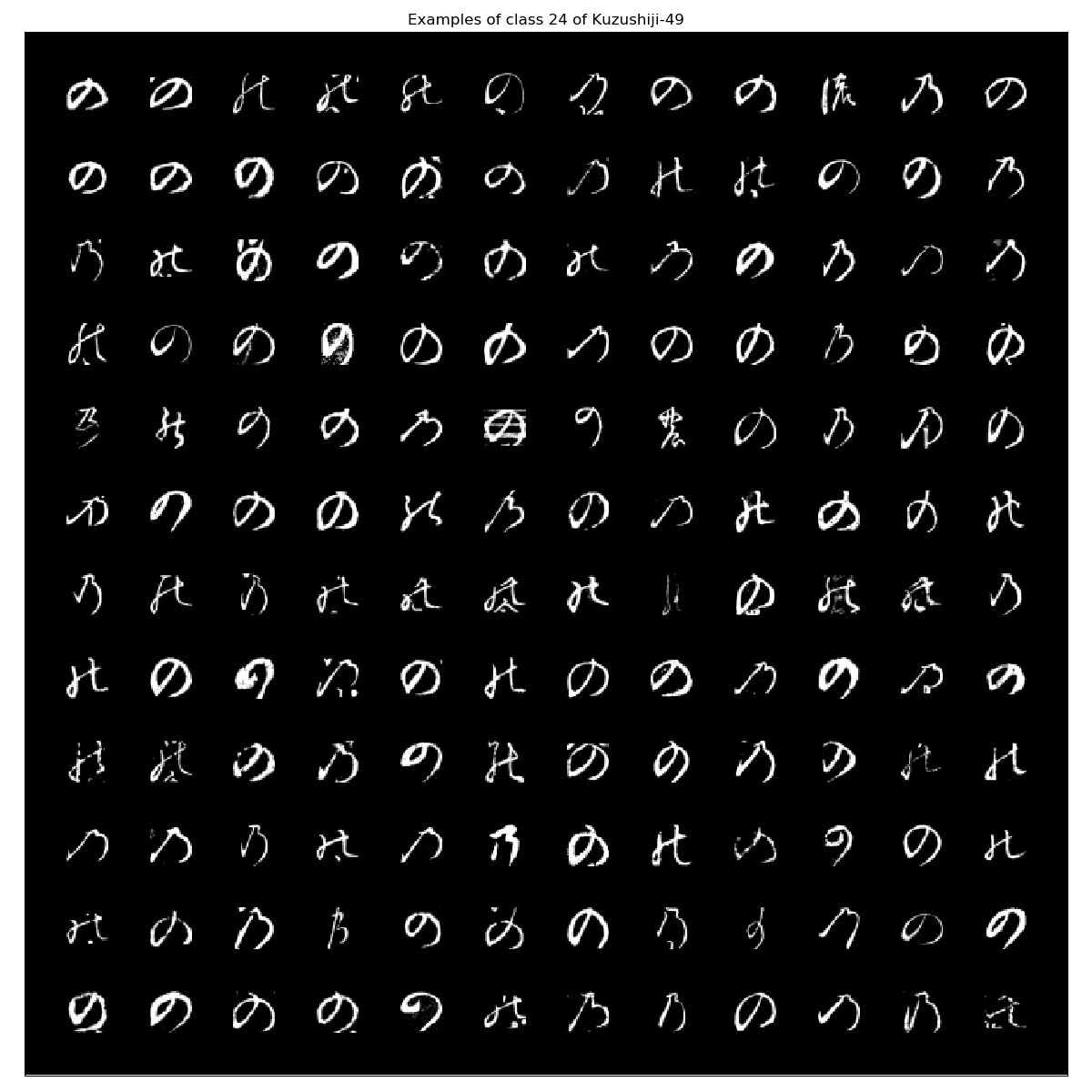
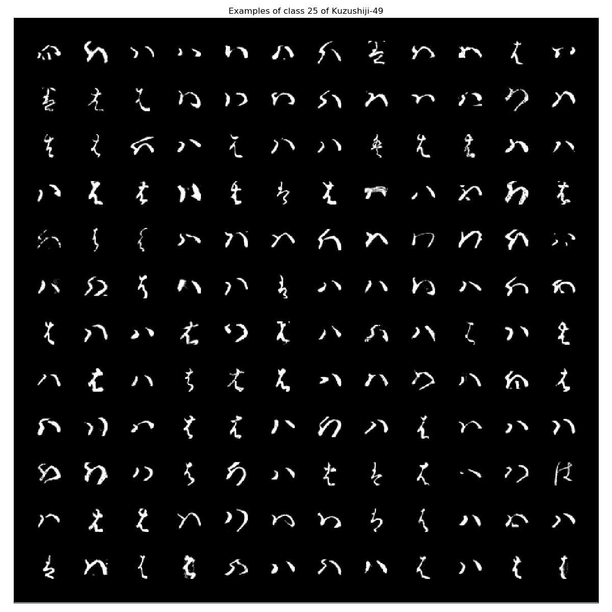
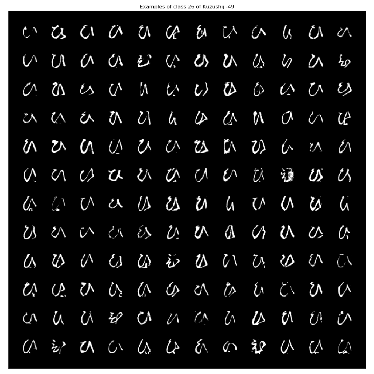
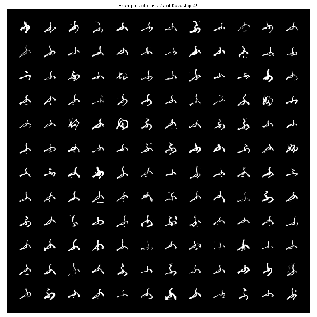
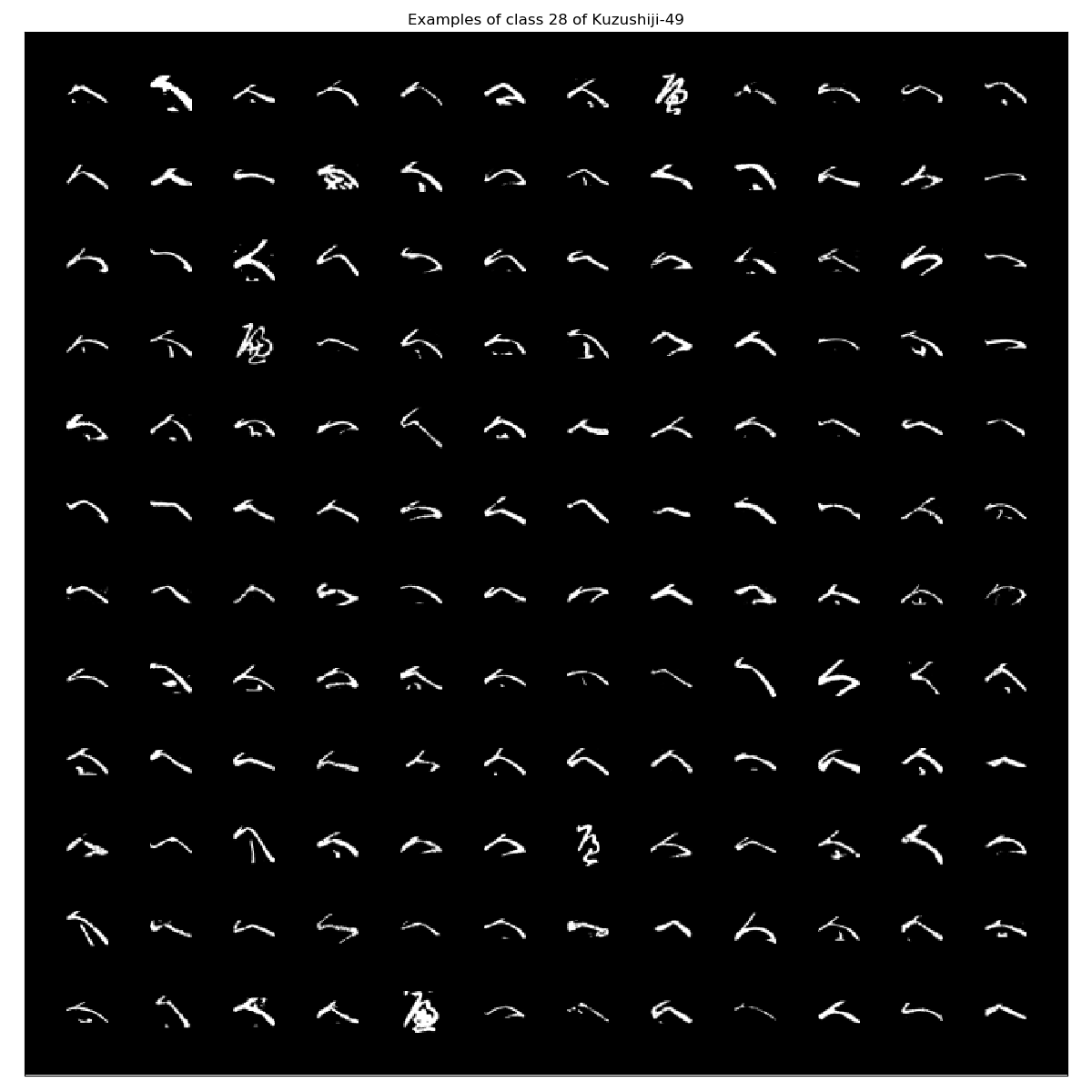
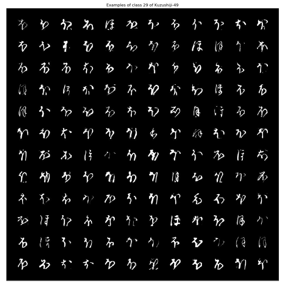
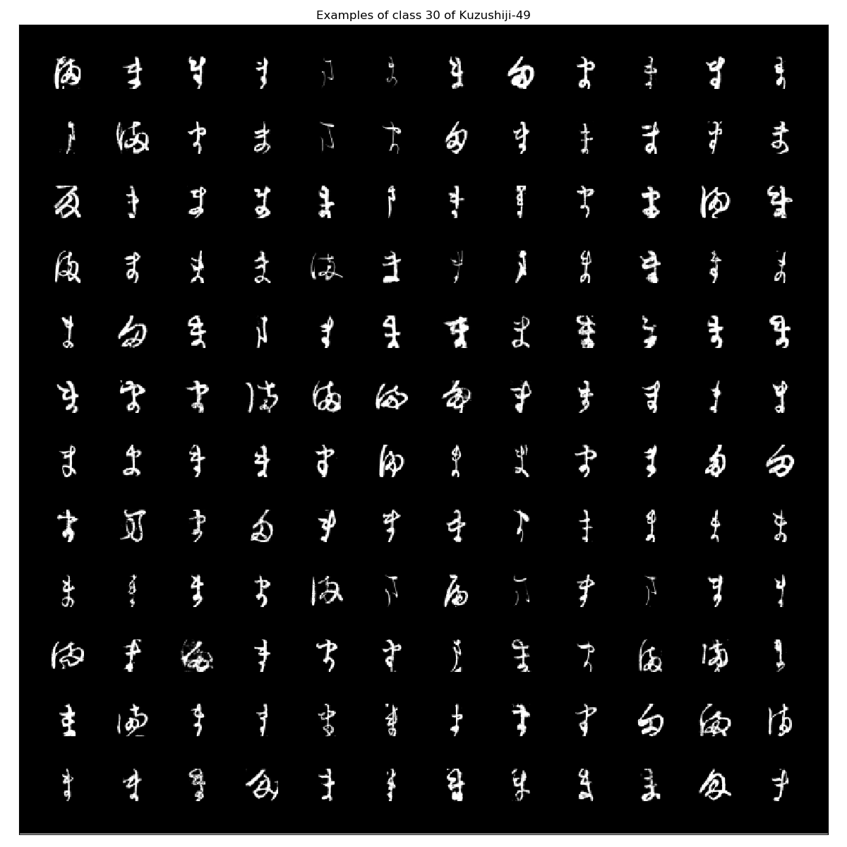
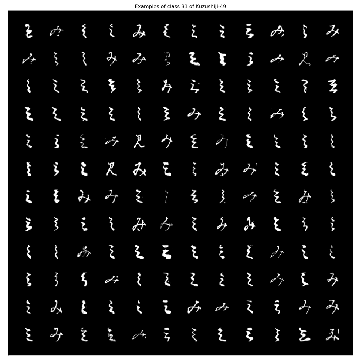
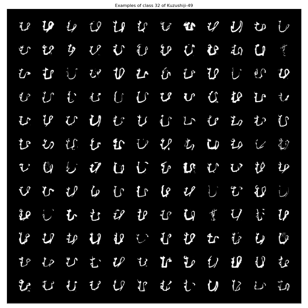
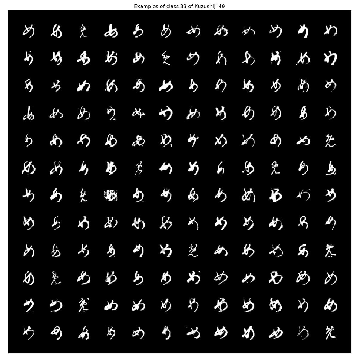
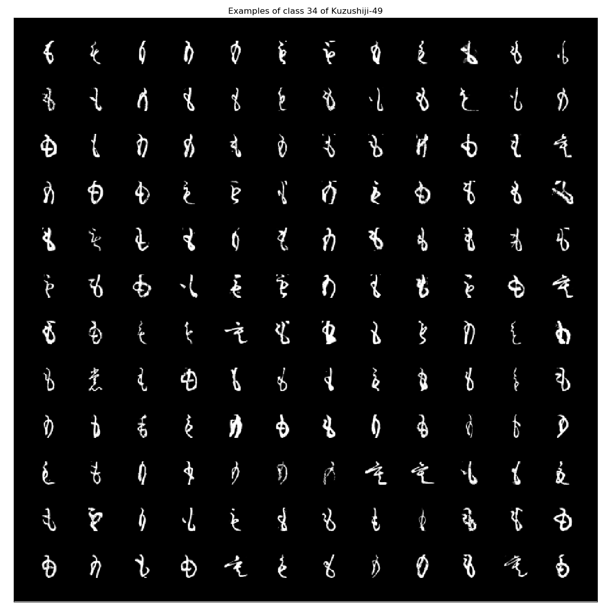

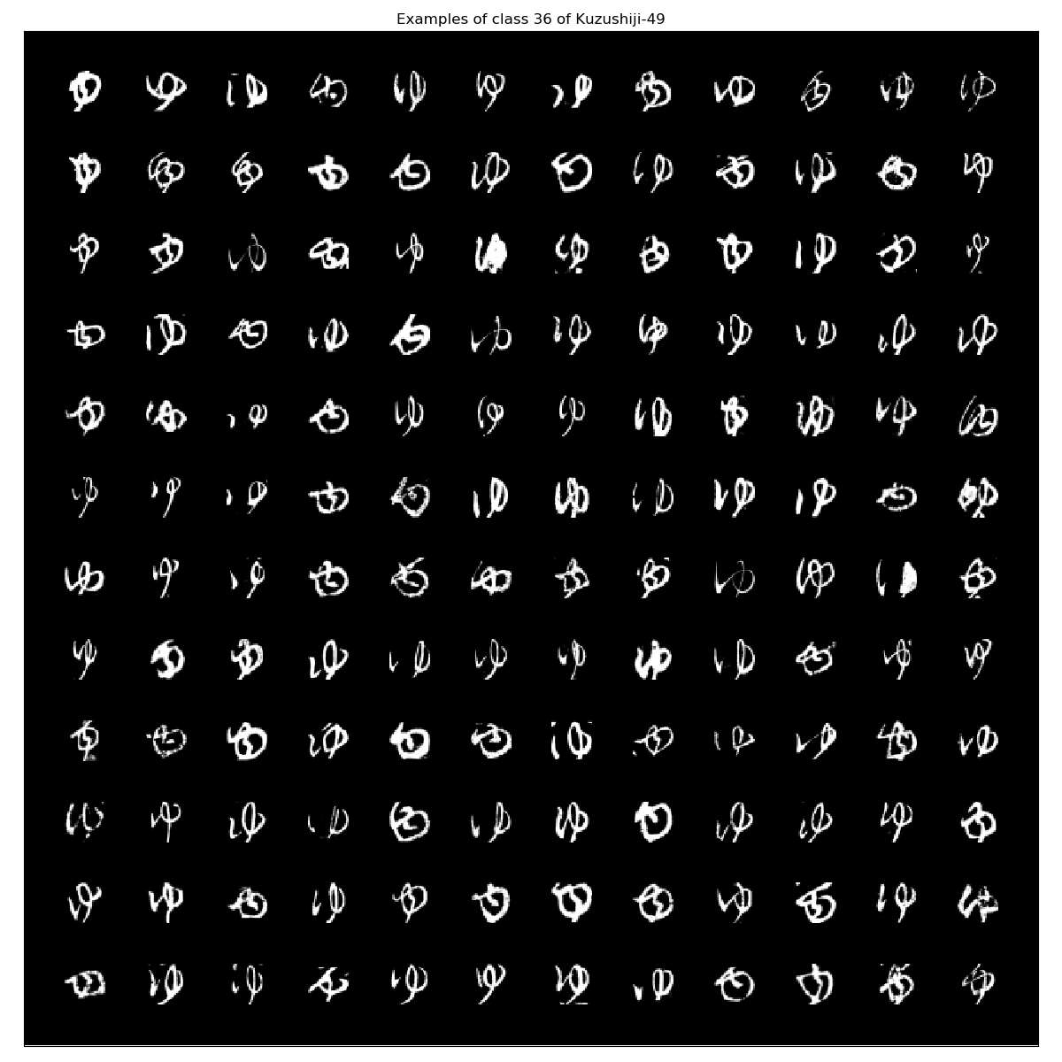
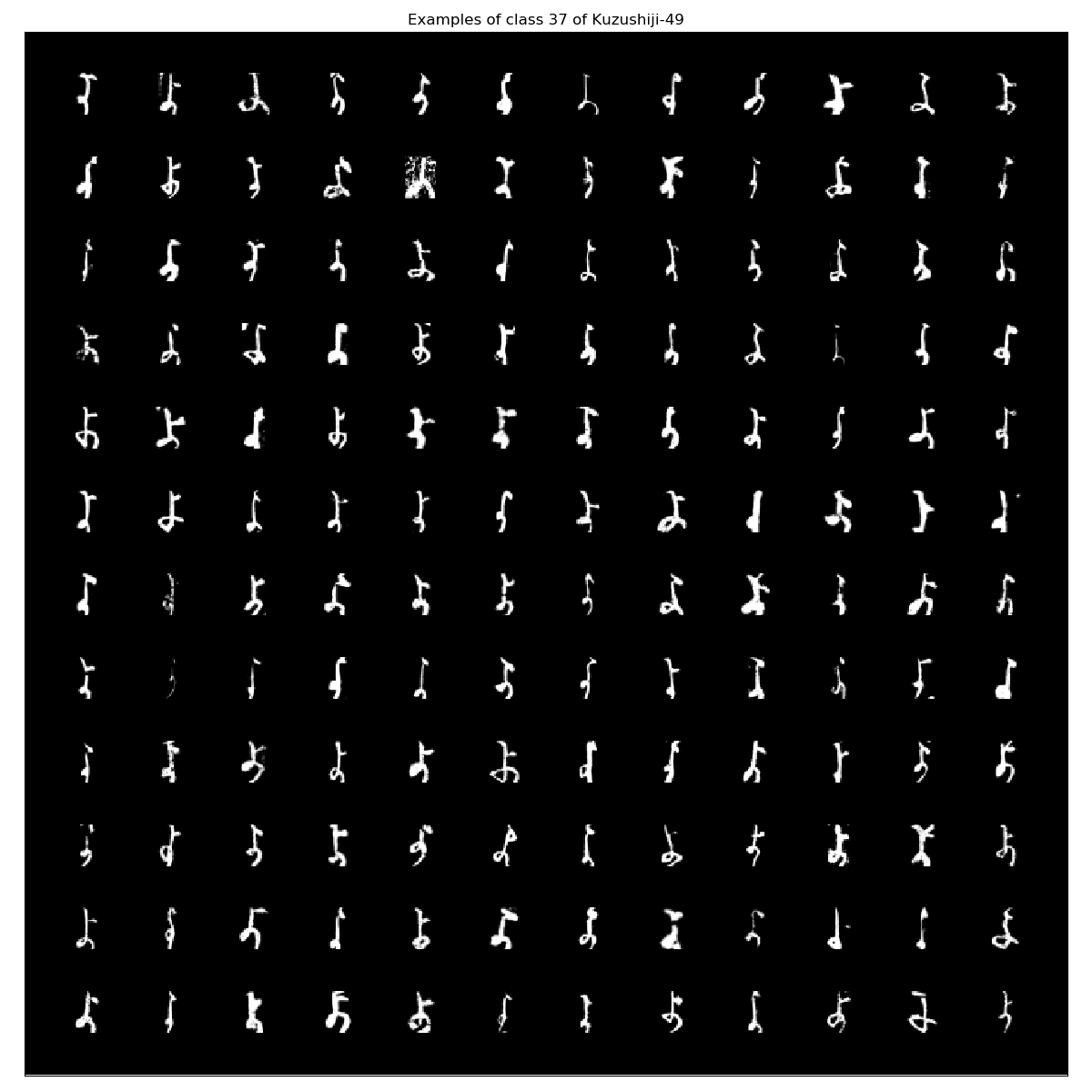
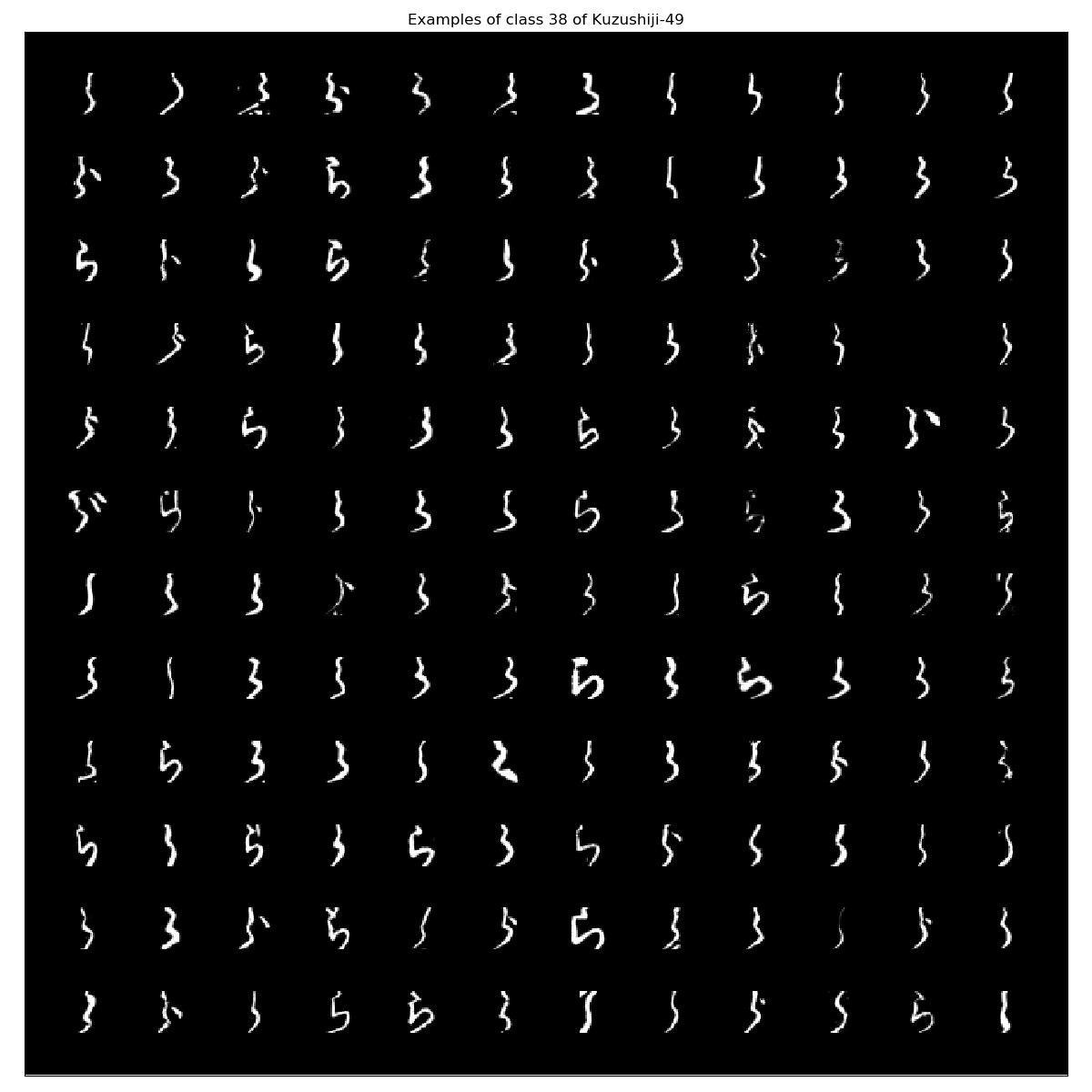
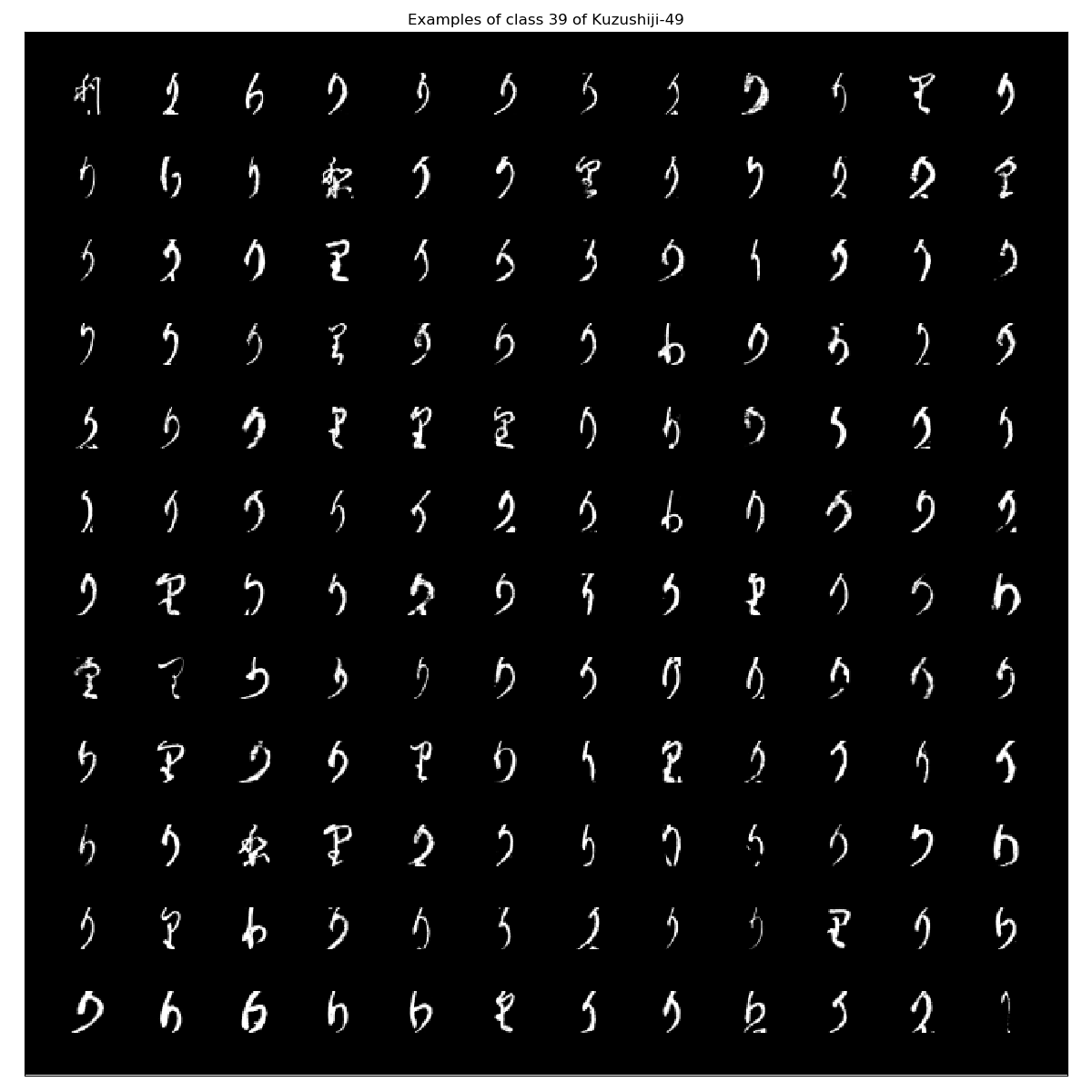
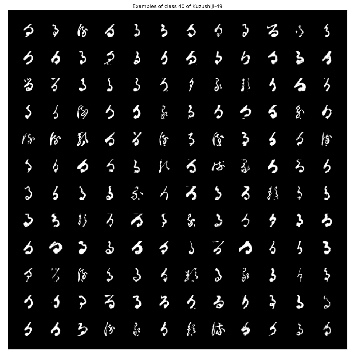
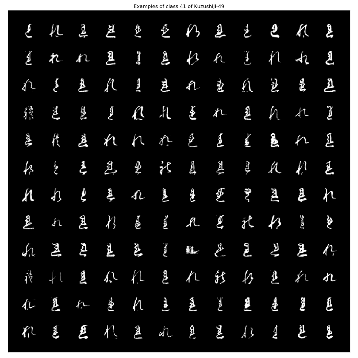
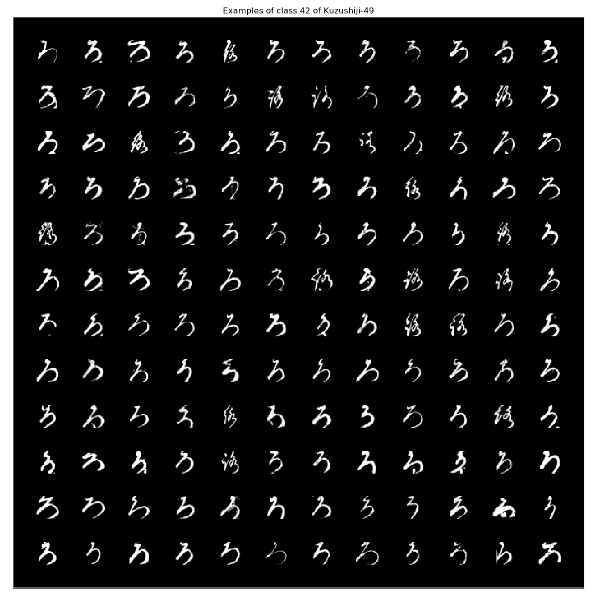
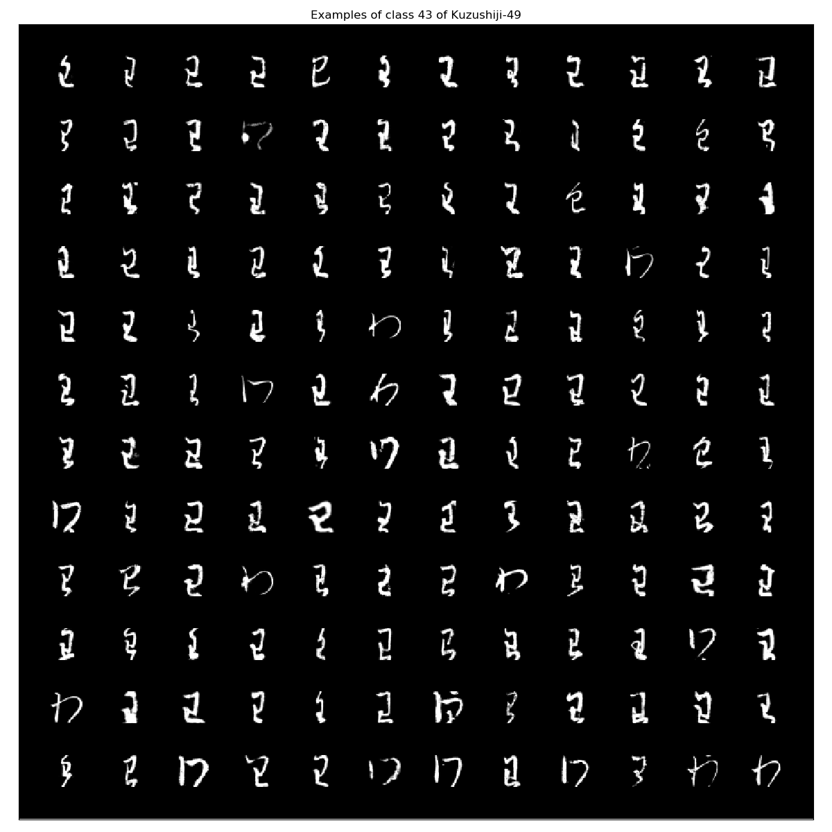
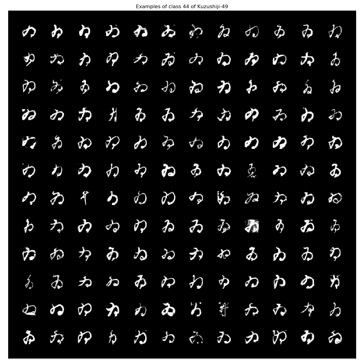

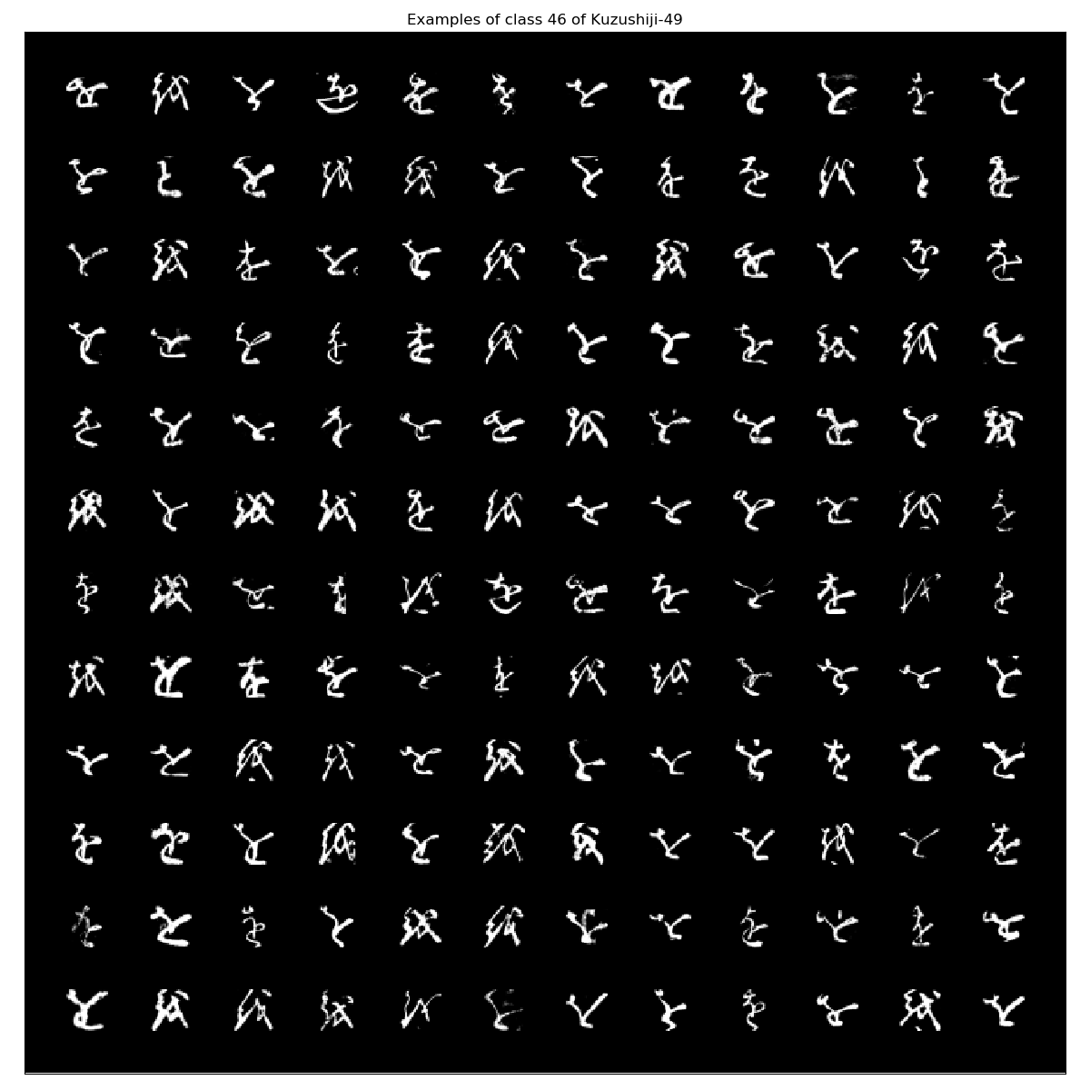
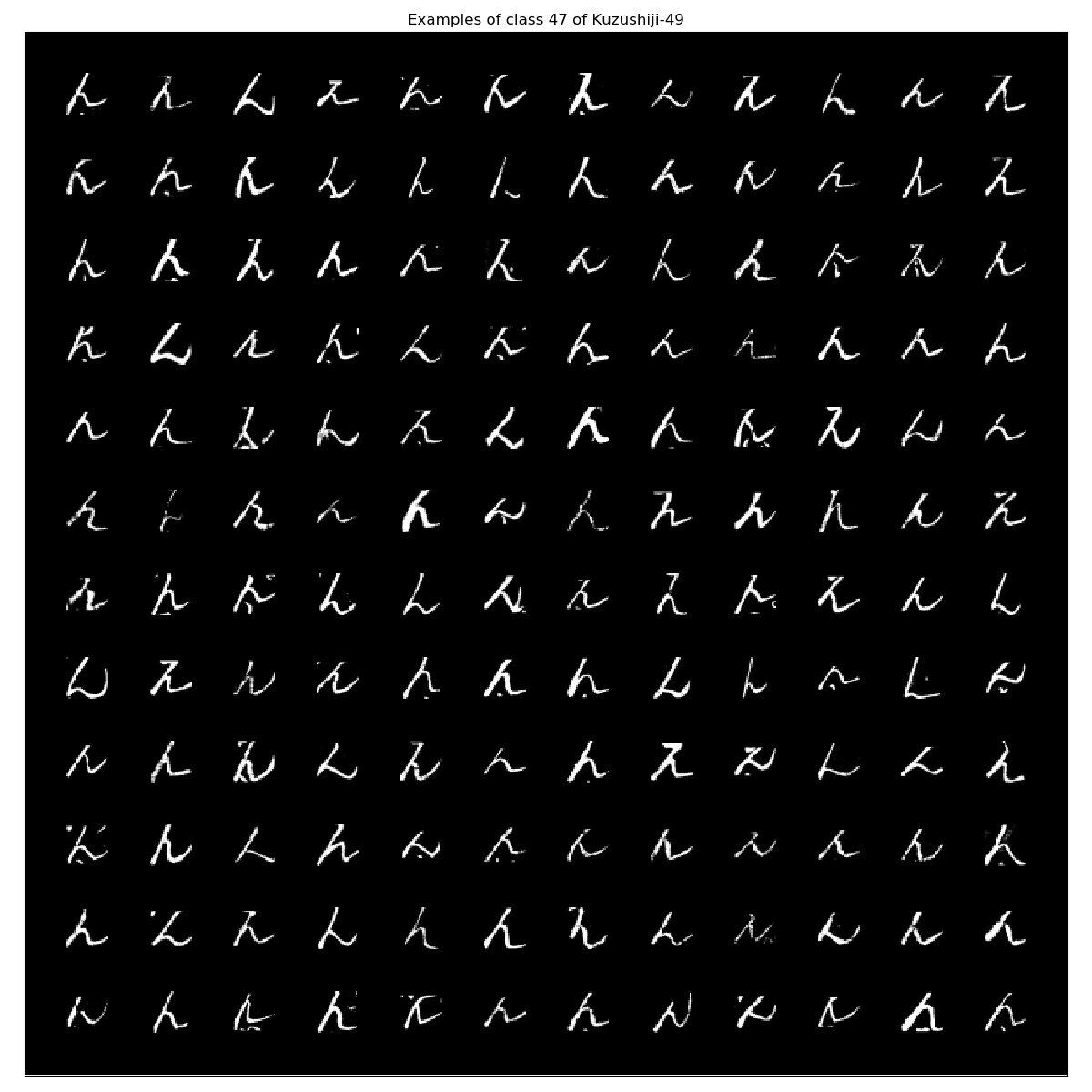
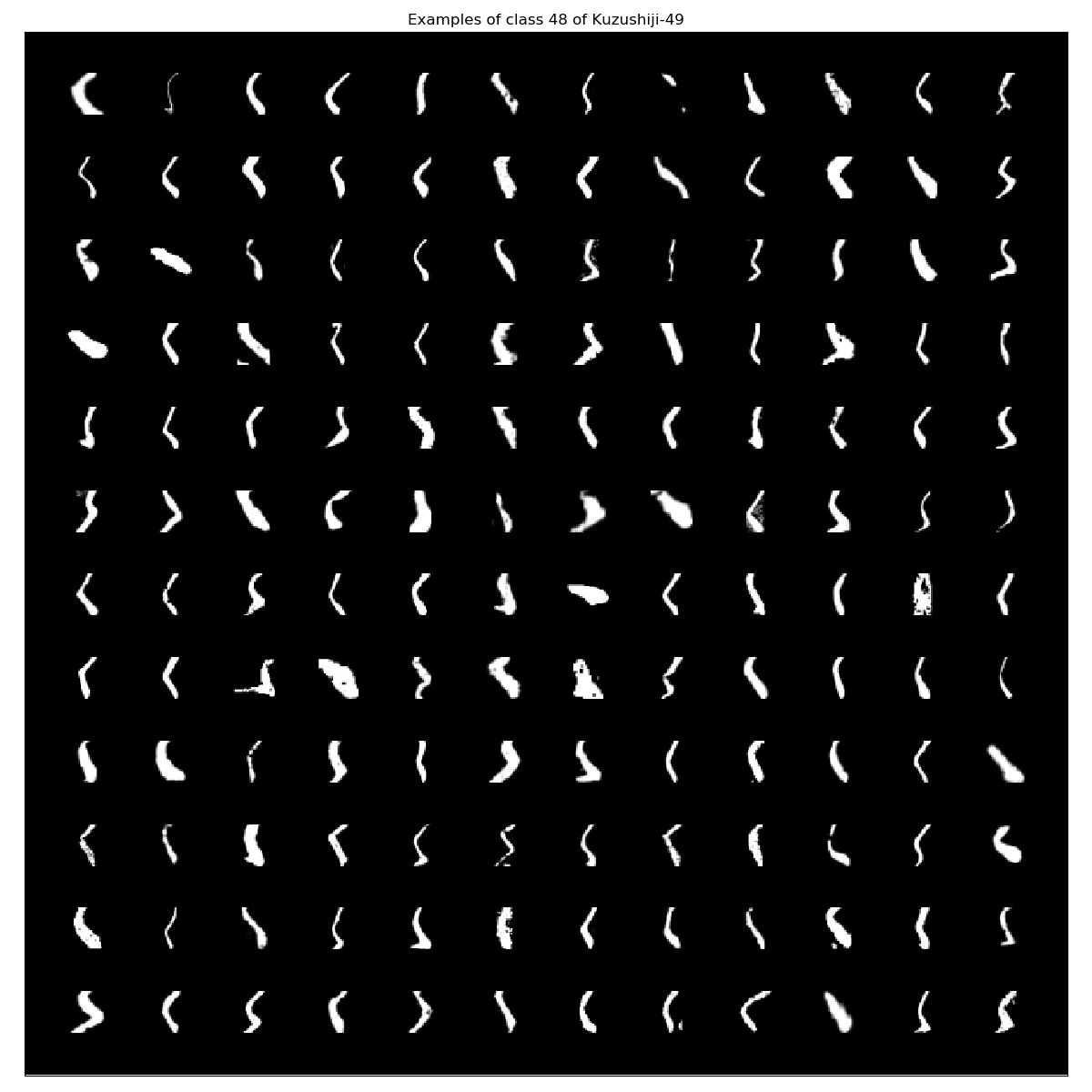
From my point of there are some images that could be misclassified. However, besides detecting basic shapes they all look alike to mee.
Kuzushiji-Kanji
The third benchmark dataset that is provided is the Kuzushiji-Kanji. These images are no longer 28x28 but 64x64 grayscale images. It contains 140426 images of 3832 classes in total. There is no train-test splitting available. The unpacked dataset looks like this:
tree .
.
├── U+241C6
│   ├── 689fa55040ec4f03.png
│   └── c0d603c6ce4a4538.png
├── U+24FA3
│   ├── 4190e728bfc948e0.png
│   └── 80582798ed70ce7c.png
├── U+25DA1
│   └── 512d7fcacddd25fd.png

...

└── U+FA5C
    ├── 15e2060396eba2b3.png
    └── 679e4b2f026f6297.png

3832 directories, 140424 files
We can see that most characters have only a few examples per class:
function ReadFilePaths(PathToDataFolder)
    OutputDict = Dict{String,Array{String,1}}()
    SymbolFolders = readdir(PathToDataFolder);
    for SymbolFolder in SymbolFolders
        OutputDict[SymbolFolder] = readdir(PathToDataFolder * SymbolFolder)
    end
    return OutputDict
end

function getClassCountKanji(FilePaths, XLabel="Class", YLabel="Frequency")
    FrequencyCountDict = Dict{String,Int64}();
    for Symbol in collect(keys(Kuzushiji_Kanji_SymbolsWithFilePaths))
        FrequencyCountDict[Symbol] = size(Kuzushiji_Kanji_SymbolsWithFilePaths[Symbol])[1]
    end
    return FrequencyCountDict
end

Kuzushiji_Kanji_SymbolsWithFilePaths = ReadFilePaths(PathToDataFolder);
collect(values(getClassCountKanji(Kuzushiji_Kanji_SymbolsWithFilePaths)))
Let’s have a look at an example image per class. Therefore, we have to write a new function that uses PyPlot again:
function KanjiExamplePlots(InputDict, NumberofXSubPlots)
    DictLength = length(InputDict);
    PlotXDim = NumberofXSubPlots*2 + 1;
    PlotYDim = 2 * div(DictLength,NumberofXSubPlots);
    PyPlot.figure(figsize=(PlotXDim, PlotYDim));
    PositionCounter = 1;
    for Symbol in collect(keys(InputDict))
        PyPlot.subplot(convert(Int64,ceil(div(DictLength,NumberofXSubPlots))+1), NumberofXSubPlots, PositionCounter)
        PyPlot.imshow(convert(Array{Float64,2},Images.load(PathToDataFolder*Symbol*"/"*InputDict[Symbol][1])),
            cmap="gray")
        PyPlot.title("Example of "*Symbol)
        PyPlot.xticks([])
        PyPlot.yticks([])
        PositionCounter += 1
    end
    PyPlot.tight_layout()
    PyPlot.savefig("./graphics/KanjiExamples.png")
    PyPlot.close()
end


KanjiExamplePlots(Kuzushiji_Kanji_SymbolsWithFilePaths,15)

A train/test split version should be released in near future. Further, it contains a few black images as well. I’ll provide some baseline results once train-test splits are released.
Benchmark models
The dataset comes with two
Benchmarks models. The first is a 4-Nearest Neighbors and the second a very simple convolutional neural network:
# kNN with neighbors=4 benchmark for Kuzushiji-MNIST
# Acheives 97.4% test accuracy

from sklearn.neighbors import KNeighborsClassifier
import numpy as np

def load(f):
    return np.load(f)['arr_0']

# Load the data
x_train = load('kuzushiji10-train-imgs.npz')
x_test = load('kuzushiji10-test-imgs.npz')
y_train = load('kuzushiji10-train-labels.npz')
y_test = load('kuzushiji10-test-labels.npz')

# Flatten images
x_train = x_train.reshape(-1, 784)
x_test = x_test.reshape(-1, 784)

clf = KNeighborsClassifier(n_neighbors=4, weights='distance', n_jobs=-1)
print('Fitting', clf)
clf.fit(x_train, y_train)
print('Evaluating', clf)

test_score = clf.score(x_test, y_test)
print('Test accuracy:', test_score)
# Based on MNIST CNN from Keras' examples: https://github.com/keras-team/keras/blob/master/examples/mnist_cnn.py (MIT License)

from __future__ import print_function
import keras
from keras.models import Sequential
from keras.layers import Dense, Dropout, Flatten
from keras.layers import Conv2D, MaxPooling2D
from keras import backend as K
import numpy as np

batch_size = 128
num_classes = 10
epochs = 12

# input image dimensions
img_rows, img_cols = 28, 28

def load(f):
    return np.load(f)['arr_0']

# Load the data
x_train = load('kuzushiji10-train-imgs.npz')
x_test = load('kuzushiji10-test-imgs.npz')
y_train = load('kuzushiji10-train-labels.npz')
y_test = load('kuzushiji10-test-labels.npz')

if K.image_data_format() == 'channels_first':
    x_train = x_train.reshape(x_train.shape[0], 1, img_rows, img_cols)
    x_test = x_test.reshape(x_test.shape[0], 1, img_rows, img_cols)
    input_shape = (1, img_rows, img_cols)
else:
    x_train = x_train.reshape(x_train.shape[0], img_rows, img_cols, 1)
    x_test = x_test.reshape(x_test.shape[0], img_rows, img_cols, 1)
    input_shape = (img_rows, img_cols, 1)

x_train = x_train.astype('float32')
x_test = x_test.astype('float32')
x_train /= 255
x_test /= 255
print('{} train samples, {} test samples'.format(len(x_train), len(x_test)))

# Convert class vectors to binary class matrices
y_train = keras.utils.to_categorical(y_train, num_classes)
y_test = keras.utils.to_categorical(y_test, num_classes)

model = Sequential()
model.add(Conv2D(32, kernel_size=(3, 3),
                 activation='relu',
                 input_shape=input_shape))
model.add(Conv2D(64, (3, 3), activation='relu'))
model.add(MaxPooling2D(pool_size=(2, 2)))
model.add(Dropout(0.25))
model.add(Flatten())
model.add(Dense(128, activation='relu'))
model.add(Dropout(0.5))
model.add(Dense(num_classes, activation='softmax'))

model.compile(loss=keras.losses.categorical_crossentropy,
              optimizer=keras.optimizers.Adadelta(),
              metrics=['accuracy'])

model.fit(x_train, y_train,
          batch_size=batch_size,
          epochs=epochs,
          verbose=1,
          validation_data=(x_test, y_test))

train_score = model.evaluate(x_train, y_train, verbose=0)
test_score = model.evaluate(x_test, y_test, verbose=0)
print('Train loss:', train_score[0])
print('Train accuracy:', train_score[1])
print('Test loss:', test_score[0])
print('Test accuracy:', test_score[1])
I’m not so sure what’s wrong nowadays but it seems like most people are neglecting proper train-valid-test splitting again after cross-validation became a bit more popular due to the recent machine learning hype. This dataset is far from big enough to neglect a validation set.
It’s time to run some fast and simple models but with proper train-valid-test splitting.
Benchmark models - Kuzushiji-MNIST
Their baseline results on the testing set are:
| Model | MNIST | Kuzushiji-MNIST | Kuzushiji-49 |
|---|---|---|---|
| 4-Nearest Neighbour Baseline | 97.14% | 91.56% | 86.01% |
| Keras Simple CNN Benchmark | 99.06% | 95.12% | 89.25% |
I’m not going to compare it to MNIST!
import ScikitLearn
import Flux
4-NN on Kuzushiji-MNIST
Well, lets be a tiny bit more creative here and not limit k-NN to 4 ;).
# dataset in 1D for ScikitLearn
Kuzushiji_MNIST_X_train_flat = reshape(Kuzushiji_MNIST_X_train, (size(Kuzushiji_MNIST_X_train)[1],size(Kuzushiji_MNIST_X_train)[2]*size(Kuzushiji_MNIST_X_train)[3]));
Kuzushiji_MNIST_X_test_flat = reshape(Kuzushiji_MNIST_X_test, (size(Kuzushiji_MNIST_X_test)[1],size(Kuzushiji_MNIST_X_test)[2]*size(Kuzushiji_MNIST_X_test)[3]));

ScikitLearn.@sk_import neighbors: KNeighborsClassifier;
GridSCV = ScikitLearn.GridSearch.GridSearchCV;


KNNClassifier = KNeighborsClassifier(n_jobs=-1)
GridParameters = Dict{String, Array}(
    "n_neighbors" => [3 4 5 6 7 8 9],
    "weights" => ["uniform", "distance"],
    "algorithm" => ["ball_tree", "kd_tree", "brute"],
    "leaf_size" => [15 30 45 60],
    "p" => [1 2 3 4 5] #using Manhattan distance (1), Euclidean distance (2), arbitray Minkowski distances
    );
GridObject = GridSCV(
    KNNClassifier,
    GridParameters,
    cv=5,
    verbose=2
    # n_jobs=-1 is not implemented yet :(
    );
GridFit = ScikitLearn.fit!(
    GridObject,
    Kuzushiji_MNIST_X_train_flat,
    Kuzushiji_MNIST_y_train
    )
That is what I intended to run. However, it turned out to be really slow on a slighly old notebook. Hence, I ran this reduced version I’ll post the proper results once I’m back home and have access to my workstation again:
KNNClassifier = KNeighborsClassifier(n_jobs=-1)
GridParameters = Dict{String, Array}(
    "n_neighbors" => [3 4],#[3 4 5 6 7 8 9],
    #"weights" => #["uniform", "distance"],
    #"algorithm" => #["ball_tree", "kd_tree", "brute"],
    #"leaf_size" => #[15 30 45 60],
    "p" => [1 2]#[1 2 3 4 5] #using Manhattan distance (1), Euclidean distance (2), arbitray Minkowski distances
    );
GridObject = GridSCV(
    KNNClassifier,
    GridParameters,
    cv=5,
    verbose=2,
    # n_jobs=-1 is not implemented yet :(
    );
GridFit = ScikitLearn.fit!(
    GridObject,
    Kuzushiji_MNIST_X_train_flat,
    Kuzushiji_MNIST_y_train
    )
Fitting 5 folds for each of 4 candidates, totalling 20 fits
[CV] n_neighbors=3, p=1
[CV] n_neighbors=3, p=1  -  617.4s
[CV] n_neighbors=3, p=1
[CV] n_neighbors=3, p=1  -  568.3s
[CV] n_neighbors=3, p=1
[CV] n_neighbors=3, p=1  -  527.4s
[CV] n_neighbors=3, p=1
[CV] n_neighbors=3, p=1  -  546.8s
[CV] n_neighbors=3, p=1
[CV] n_neighbors=3, p=1  -  467.9s
[CV] n_neighbors=3, p=2
[CV] n_neighbors=3, p=2  -  628.5s
[CV] n_neighbors=3, p=2
[CV] n_neighbors=3, p=2  -  627.2s
[CV] n_neighbors=3, p=2
[CV] n_neighbors=3, p=2  -  614.4s
[CV] n_neighbors=3, p=2
[CV] n_neighbors=3, p=2  -  612.5s
[CV] n_neighbors=3, p=2
[CV] n_neighbors=3, p=2  -  631.3s
[CV] n_neighbors=4, p=1
[CV] n_neighbors=4, p=1  -  496.8s
[CV] n_neighbors=4, p=1
[CV] n_neighbors=4, p=1  -  609.4s
[CV] n_neighbors=4, p=1
[CV] n_neighbors=4, p=1  -  620.5s
[CV] n_neighbors=4, p=1
[CV] n_neighbors=4, p=1  -  555.7s
[CV] n_neighbors=4, p=1
[CV] n_neighbors=4, p=1  -  489.0s
[CV] n_neighbors=4, p=2
[CV] n_neighbors=4, p=2  -  575.9s
[CV] n_neighbors=4, p=2
[CV] n_neighbors=4, p=2  -  500.7s
[CV] n_neighbors=4, p=2
[CV] n_neighbors=4, p=2  -  480.4s
[CV] n_neighbors=4, p=2
[CV] n_neighbors=4, p=2  -  521.8s
[CV] n_neighbors=4, p=2
[CV] n_neighbors=4, p=2  -  561.0s

ScikitLearn.Skcore.GridSearchCV
  estimator: PyCall.PyObject
  param_grid: Dict{String,Array}
  scoring: Nothing nothing
  loss_func: Nothing nothing
  score_func: Nothing nothing
  fit_params: Dict{Any,Any}
  n_jobs: Int64 1
  iid: Bool true
  refit: Bool true
  cv: Int64 5
  verbose: Int64 2
  error_score: String "raise"
  scorer_: ScikitLearnBase.score (function of type typeof(ScikitLearnBase.score))
  best_params_: Dict{Symbol,Any}
  best_score_: Float64 0.9625166666666667
  grid_scores_: Array{ScikitLearn.Skcore.CVScoreTuple}((4,))
  best_estimator_: PyCall.PyObject
That was slow…
GridFit.best_params_
Dict{Symbol,Any} with 2 entries:
  :n_neighbors => 3
  :p           => 2
Let’s predict the test set and evaluate it:
Kuzushiji_MNIST_y_test_pred = ScikitLearn.predict(GridFit,Kuzushiji_MNIST_X_test_flat);
Kuzushiji_MNIST_accuracy = sum(Kuzushiji_MNIST_y_test_pred .== Kuzushiji_MNIST_y_test)/length(Kuzushiji_MNIST_y_test_pred)
This yields an accuracy of 0.912 which is pretty close to the reference result of 91.56 %. However, our model here is properly cross-validated and therefore we can assume that it is a bit more robust.
Brute-force collection on Kuzushiji-MNIST
This one is still with Python since I didn’t had any time to convert it to Julia so far. I guess I should rewrite some things properly as well since it had grown organically for quite some time now.
Since the original brute-force pipeline required >40 h!!!, I’m going to run a rather reduced version of this here.
Benchmark models - Kuzushiji-49
4-NN on Kuzushiji-49
Will be delivered in a few days since my notebook is to slow for this.
Brute-force collection on Kuzushiji-49
This one is still with Python since I didn’t had any time to convert it to Julia so far. I guess I should rewrite some things properly as well since it had grown organically for quite some time now.
Since the original brute-force pipeline required >40 h!!!, I’m going to run a rather reduced version of this here.
References
[1] Clanuwat, T.; Bober-Irizar, M.; Kitamoto, A.; Lamb, A.; Yamamoto, K.; Ha, D. (2018): Deep Learning for Classical Japanese Literature. Neural Information Processing Systems 2018 Workshop on Machine Learning for Creativity and Design preprint: https://arxiv.org/abs/1812.01718

